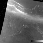
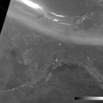
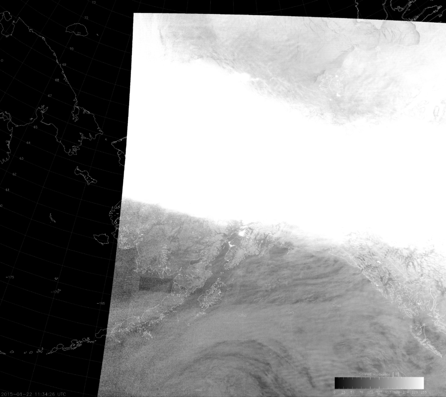
Imagine that you are an operational forecaster. (Some of you reading this don’t need to imagine it, because you are operational forecasters.) You’ve been bouncing off the walls from excitement because of all the great information the VIIRS Day/Night Band (DNB) provides. “This is so great! Visible imagery at night! It helps in so many ways,” you say to yourself or to anyone within earshot. What’s more: you read this blog and, in particular, you’ve read this blog post and/or this paper. “All our problems have been solved! We can use the DNB for any combination of sunlight and moonlight! I am so happy!” Then you come across an image like this:
If you’re short tempered, you’re thinking, “@&*!@#&#!!!” If you have better control of your emotions, you’re thinking, “Me-oh-my! Whatever happened here?” Welcome to the third installment of the seemingly-never-ending series on how difficult it is to display the highly variable DNB radiance values in an automated way.
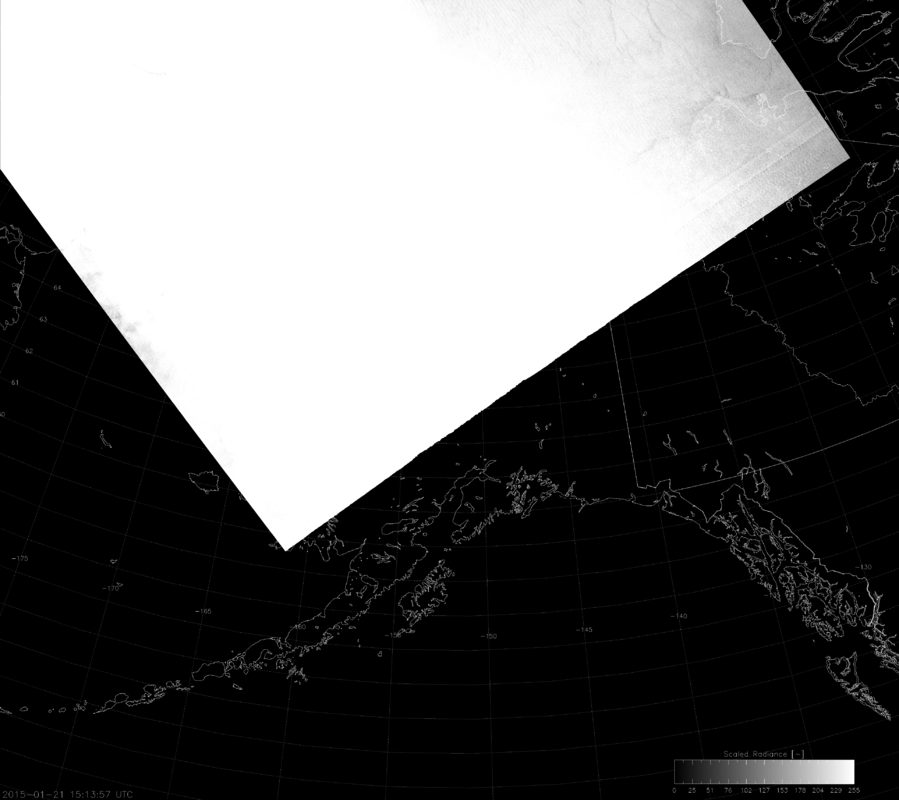
In the previous installment, which I will keep linking to until you click on it and re-read it, I outlined a great new way to scale the radiance values as a function of solar and lunar zenith angles that I call the “erf-dynamic scaling” (EDS) algorithm because it is based on the Gaussian error function (erf). This algorithm uses smooth, continuous functions to account for the 8 orders-of-magnitude variability in DNB data that occurs between day and night, and which was demonstrated to beat many previous attempts at image scaling. Unfortunately, that algorithm produced the image you see above.
So, is my algorithm a failure?
Well, if you’re going to jump right to “failure” based on this, you need to calm down and back off the hyperbole. Do you feel like a failure every time you make a mistake? Besides, mistakes are opportunities for learning.
My demonstration of the quality of the EDS method was based on images taken near the summer solstice. Now, we’re a month after winter solstice. And you know what happens in the winter that doesn’t happen in the summer? The aurora! (Actually, the aurora is present just as much in the summer, but you can’t see it because the sun is still shining.) Now that the nights are so long and dark, the aurora is easily visible.
My EDS method accounts for sunlight and moonlight. It doesn’t account for auroras and they can be several orders of magnitude brighter than the moonlight – especially near new moon when there is no moonlight. And guess when the image above was taken relative to the lunar cycle.
Now, I knew auroras would mess up my scaling algorithm (“Oh, sure you did!”), but I underestimated their occurrence. As a “Lower-48er,” I’ve seen the aurora once in my life. But, at high latitudes (*cough* Alaska *cough*) they happen almost every night in the winter. They’re not always visible due to clouds, but you can’t call them a “rare occurrence”.
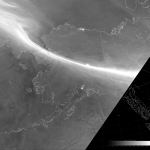
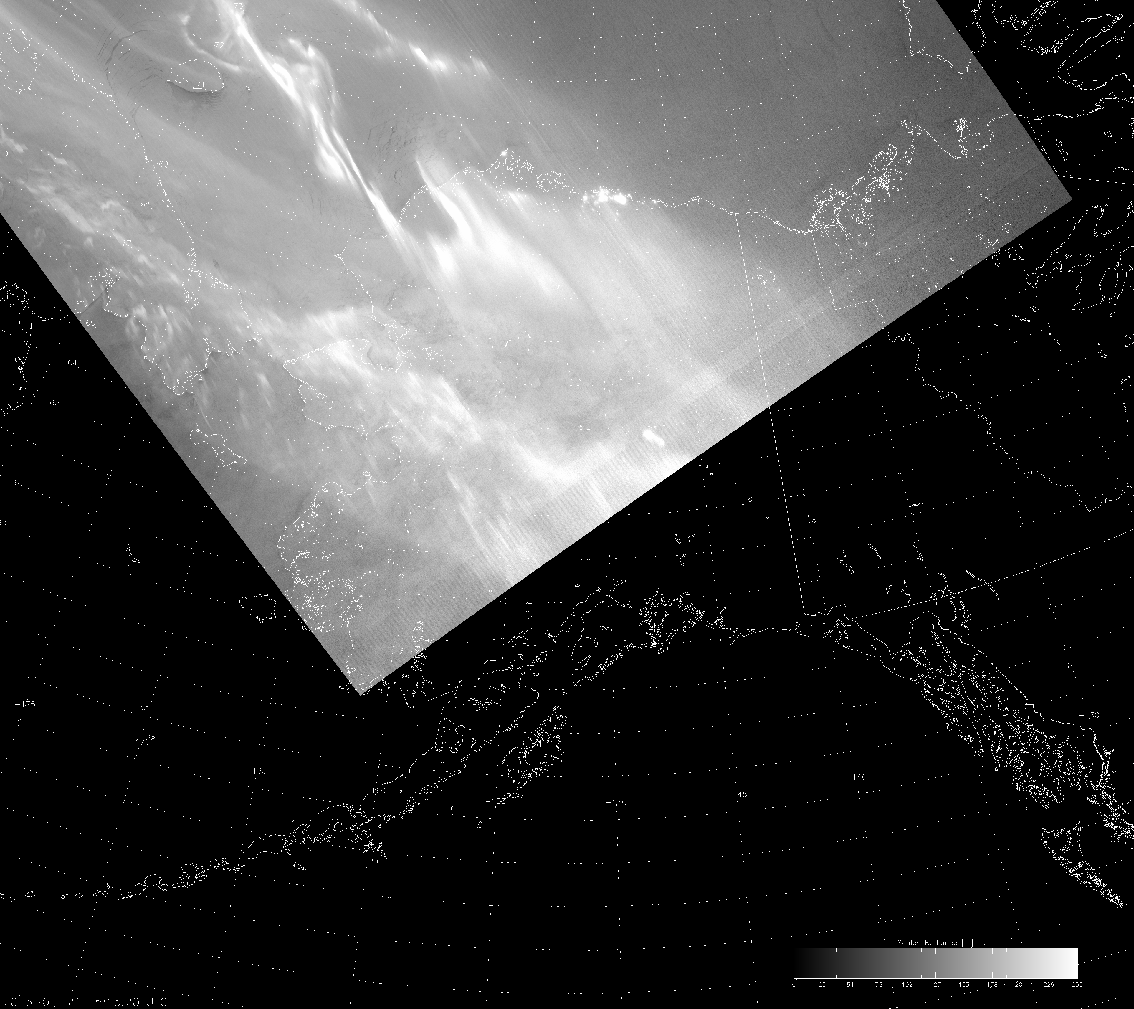
From the perspective of DNB imagery, auroras can get in the way. Or, auroras can act as another illumination source to light up important surface features. Let’s look at the above image, with the data re-scaled by manually tweaking the settings in McIDAS-v:
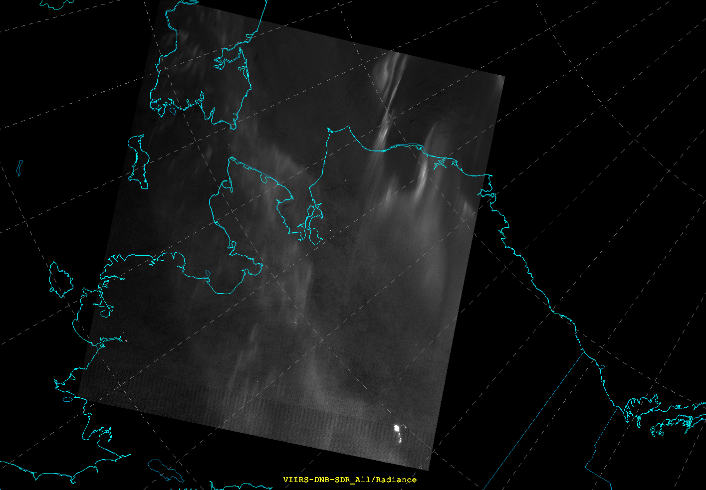
Of course, this image is rotated differently, but that’s not important. The important thing is that you can see now that it’s an aurora and you can see surface features underneath it. Cracks in the sea ice are visible! (And, remember, there is no moonlight here – just aurora and airglow.) Much better than the wall of white image, right? This proves that it’s a problem with my scaling and not with the DNB itself.
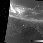
So, how do we get my scaling to work for this case? In theory, the answer is simple: bump up the max values until it’s no longer saturated. In practice, however, it’s not that simple. This was a broad, relatively diffuse aurora that was barely brighter than the max values. Some auroras are much more vivid (and much brighter than the max values), like this one:
If you increase the max values until nothing is saturated, you’ll only be able to see the brightest pixels (which are usually city lights) and nothing else. And, don’t forget: we don’t want to increase the max values everywhere all the time, because the algorithm works as-is when the aurora isn’t present (or when the moonlight is brighter than the aurora).
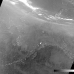
Here’s the solution: calculate max and min values with the EDS method as before, but increase the max values by 10% at a time until only a certain percentage of the image is saturated. That’s what I’ve done in the last image above, where I’ve adjusted the max values until only 0.5% of the image is saturated. In case you’re wondering, here’s the same image without this additional correction:
The correction makes it much better. What about for the first case I showed? Here’s the corrected version:
Once again, much better than before. You can see the cracks in the sea ice now! (Maybe it’s not as good as the manual scaling but, because it’s automated, it takes less time to produce. )
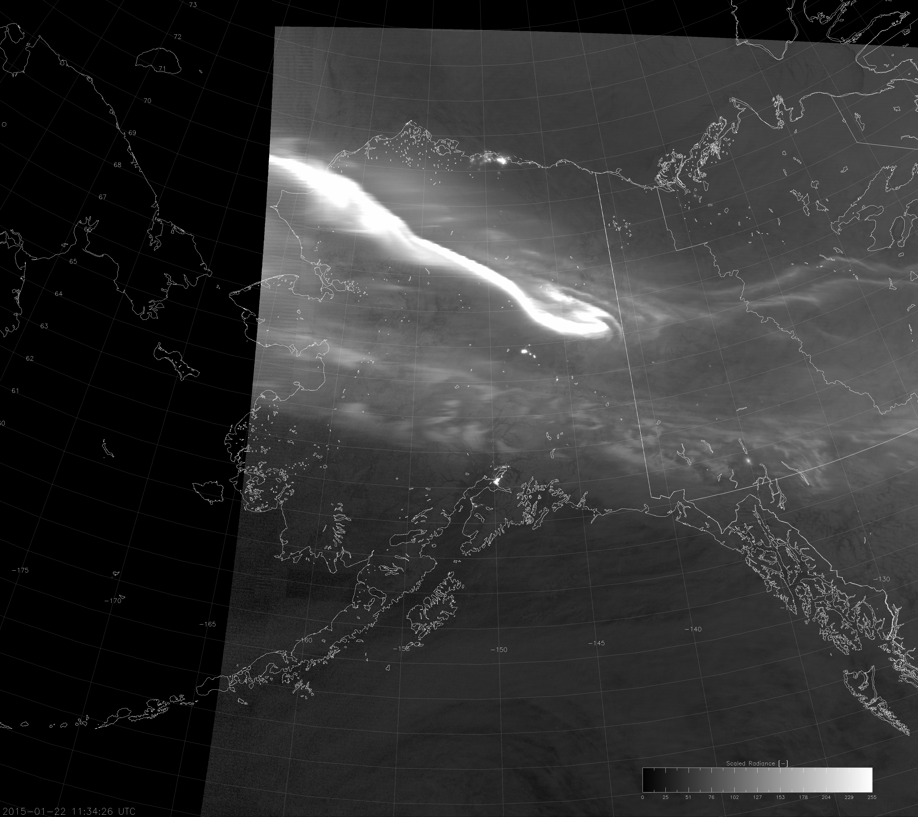
Of course, this correction assumes that less than 0.5% of the image is city lights or wildfires or lightning. And, it might not work too good if the data spans all the way from bright sunlight to new-moon night beyond the aurora because it darkens the non-aurora parts of the scene (as can be seen in the images from 22 January 2015). But, the great thing is: if the scene is not saturated by the aurora (or some other large bright feature) no correction is applied, so you still get the same great EDS algorithm results you had before.
As a bonus to make up for the initial flaws in the EDS algorithm (and to get any short-tempered viewers to stop cursing), enjoy the images below of a week’s worth of auroras as seen by the DNB (with the newly modified scaling). Make sure you look for the “Full Resolution” link to the upper right of each image in the gallery to see the full resolution version: