
While water vapor imagery is no doubt very useful for forecasting, it can at times be tricky to interpret. This blog discusses a particularly challenging case over Southern California on 21 September 2016, when deep tropical moisture produced a rain event for San Diego. Even though the environment was very moist, indeed the precipitable water (PW) was a record for the date, GOES-15 water vapor imagery (with a central wavelength of 6.7 microns) implied a “dry” atmosphere. GOES-R (now GOES-16) has 3 water vapor channels, one that senses higher in the atmosphere and the other lower than what is currently on GOES. The central wavelengths for the new water vapor channels are similar to what is currently available from the GOES-15 Sounder, and for this case we will examine all 3 channels to see how the 2 new channels compared to what we have now on GOES. Finally, we will also examine the CIRA/NESDIS Blended Total PW imagery and a new product being developed at CIRA, Blended Layered PW (LPW) imagery, to see what they reveal for this case.
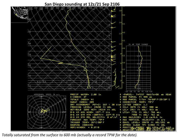
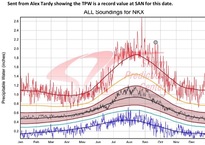
We were alerted to this case by Alex Tardy, the WCM at the San Diego WFO (SGX), who also supplied some of the graphics. Alex noted that the 12 UTC 21 Sep SAN sounding (below) had a record TPW for the date (chart below).
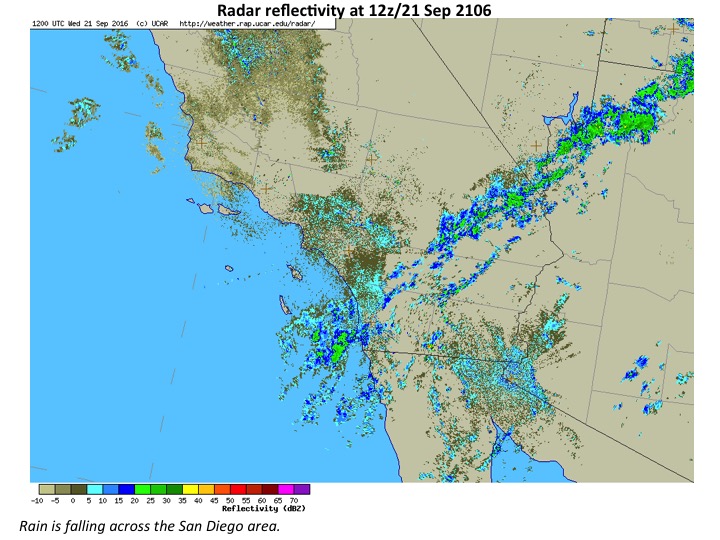
All this moisture produced widespread rain across far southern California, as depicted in the radar image shown below.
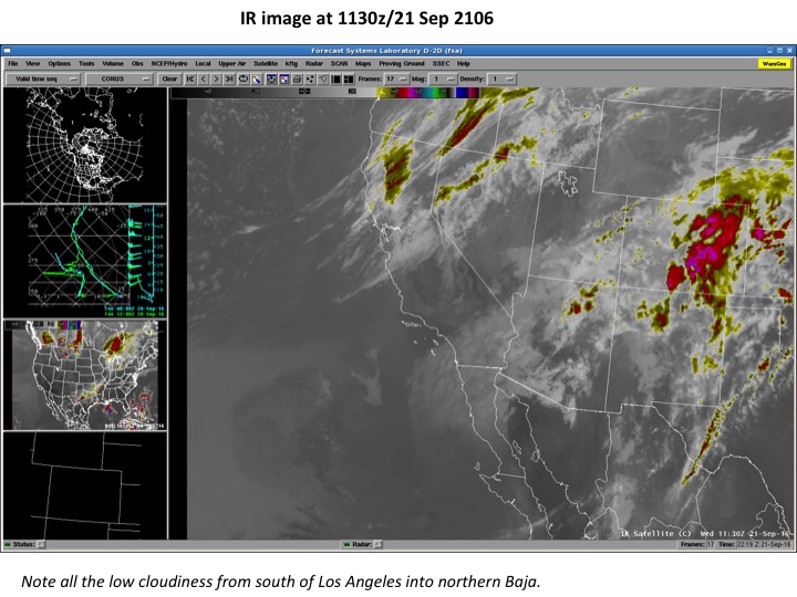
IR imagery at 1130 UTC indicates the clouds producing this rain did not extend to very high levels. Sampling of the IR temperature near SAN yields a cloud top temperature of +1C or 274K. Using the 12z SAN sounding this corresponds to a cloud top of about 580 mb.
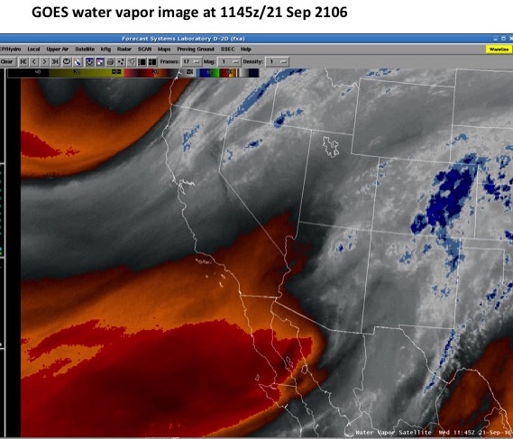
First let’s look at a water vapor image near the time of the above imagery (1145 UTC) from GOES-15, which has a single channel at 6.19 microns (μ). The weighting function (discussed further below) for the imager channel is fairly broad, extending generally from 300 to around 400 mb. Note that over San Diego and areas to the south this water vapor channel shows a large area of warm brightness temperatures, which forecasters often interpret as indicative of a dry atmosphere. The color table being used is the “RAMSDIS water vapor” table available on AWIPS2.
We can use water vapor imagery derived from the GOES-15 Sounder to get an idea what the 2 new water vapor channels that are on GOES-16 (-R) would show. While the central wavelengths of the Sounder-based water vapor imagery compare to what is on GOES-16, the resolution is of course far worse (~8 km vs 2 km), and of course not as good as what is currently on GOES (4 km). We can see this resolution difference (between GOES and the Sounder) by comparing the above image to the equivalent mid-level channel from the Sounder shown below. Besides the resolution the imagery otherwise are fairly similar.
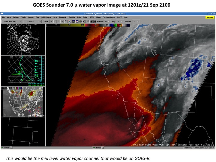 The 7.0 μ water vapor image shown above would generally sense somewhat lower in the atmosphere compared to the GOES imager water vapor image shown earlier. The next image is the upper level water vapor channel from the Sounder-based imagery, shown below for the same time (1201 UTC), which would sense vertically a little higher than the current GOES imager channel. The area of warmer brightness temperatures is not as extensive as in the mid-level imagery, indicating contribution from moisture at higher levels (the average weighting function for the 6.5 μ imagery is centered close to 300 mb for the standard atmosphere).
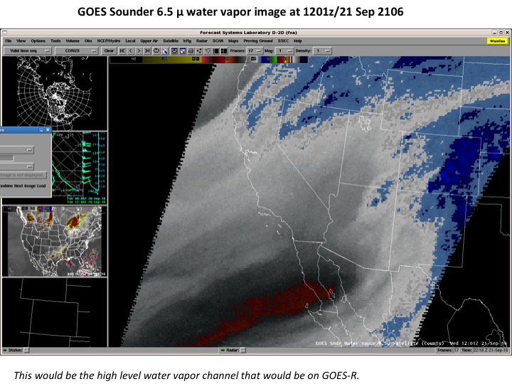
Perhaps the most intriguing of the new water vapor channels is the lower level channel, which from the Sounder would sense near 600 mb or lower. The image for 1201 UTC from this channel at 7.4 μ is shown below.
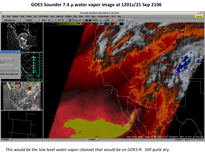
Even though this channel senses lower into the atmosphere, we still see warm brightness temperatures from the SAN area southward. These warm temperatures and by inference perhaps dry conditions are found even above an area where rain is occurring AND the environment has a record TPW level. How is this possible? To answer this question we need to look in more detail at what levels the various channels are actually sensing. Remember, the weighting functions depend on the temperature and moisture distribution in the environment, and the satellite viewing angle, and this means they will be sensing different levels across a domain. Below is what the weighting functions look like for the SAN sounding that was shown earlier.
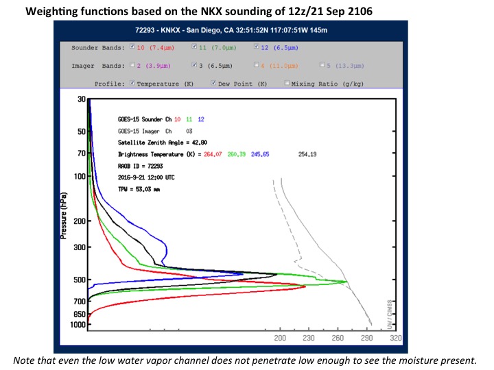
In the above figure the channel number is given for each band; Sounder Channel 10 = 7.4 μ, 11 = 7.0 μ and 12 = 6.5 μ, and the GOES imager water vapor channel is #3. The brightness temperatures that are listed in the above figure would be equivalent to what one would find using the sampling tool on AWIPS2 for the various channels when sampling over SAN.
The weighting functions above differ from what would be calculated for the “standard atmosphere”, shown in the figure below.
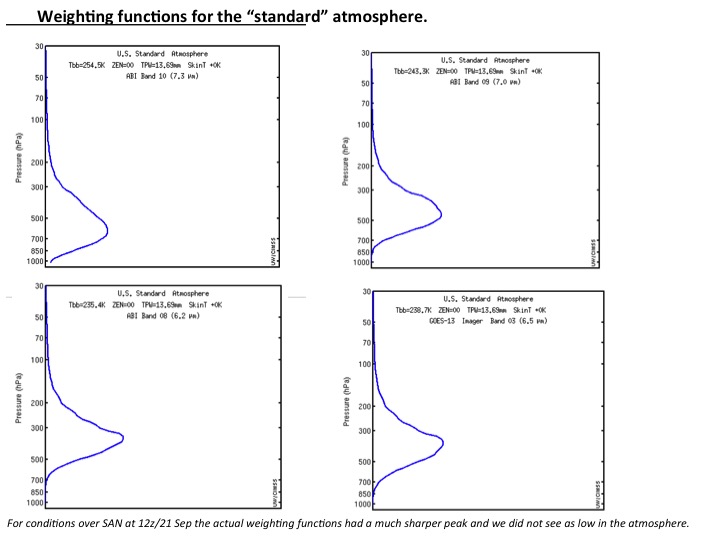
The actual weighting functions are generally narrower and more complex than those from the standard atmosphere. One important caveat to note about the weighting functions calculated for the 1200 UTC sounding is that while the viewing angle has been considered, the profiles are calculated using a forward model for clear sky conditions. In our case we know that there are overcast conditions with a cloud top temperature derived from the IR imagery of 274K or ~580 mb over the SAN area. The cloudy conditions would quickly saturate a given channel if it were to sense into the cloud layer, so there will be no contribution much below the top of the cloud layer. In our case we note that if it were clear two of the Sounder channels would penetrate below the 580 mb level, so for these two channels the presence of the cloud layer should shift the actual weighting function upwards (colder), moreso for the 7.4 μ channel compared to the 7.0 μ channel. Indeed, when we sampled these two channels over the SAN area the brightness temperatures found were 261 K for 7.4 μ and 259 K for 7.0 μ. For the lower 7.4 μ channel this is 3 K colder than the brightness temperature listed for this channel as calculated for clear sky conditions, so a shift to higher in the atmosphere, as expected. For the 7.0 μ channel the difference is only one degree, as would be expected smaller since that weighting function under clear sky conditions did not penetrate below the level where the cloud top occurred (580 mb). With this in mind, for this case there was just enough moisture in the environment above the deep moist layer to saturate even the lowest water vapor channel before it sensed down to the cloud top, so it looked relatively “dry” even though we had a record TPW present in the atmosphere.
This case shows that while the new water vapor channels will be powerful tools for forecasters, we must be careful to note that they do not necessarily tell us what the moisture profile looks like through the entire atmosphere. In other words, we cannot determine from the water vapor imagery how much PW is present in the atmosphere. There is, however, satellite imagery that does allow one to detect the actual TPW present. Most forecasters are familiar with this imagery on AWIPS2 known as the NESDIS Blended TPW product, which is shown for this case below.
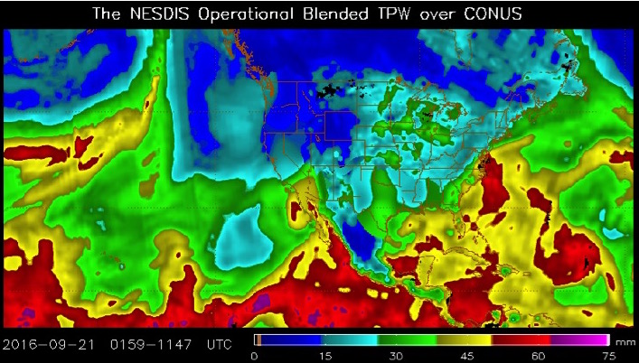
This imagery combines measurements from several Polar satellites into a single image, hence the “blended” title and the time stamp that covers a time period instead of a single time. The Polar satellites used have instruments that can measure the TPW even in the presence of clouds. What we see of course for this case is the high TPW area associated with the remnants of the tropical system just to the south of San Diego, with the higher TPW values extending to the north. We certainly get a different picture of the water vapor present in the atmosphere from this imagery compared to what we saw with the water vapor imagery. CIRA is experimenting with a variant of this product that shows the PW in different layers, with the blended product known as the Layered Precipitable Water product (LPW). The LPW for this case is shown below.
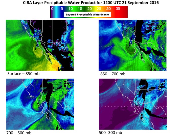
In agreement with what we saw in the San Diego 1200 UTC sounding, the LPW product shows moisture through the lower 3 layers but dry conditions above 500 mb (this higher level dry air is what was implied by the water vapor imagery). This is also a blended product and while it is labeled at 1200 UTC it actually covers several hours leading up to this time. A future version of this product will use an advective scheme that will make it more visually appealing. This product is currently being tested at some WFOs, and if you are interested contact us and we can make it available on AWIPS2 through the LDM.