
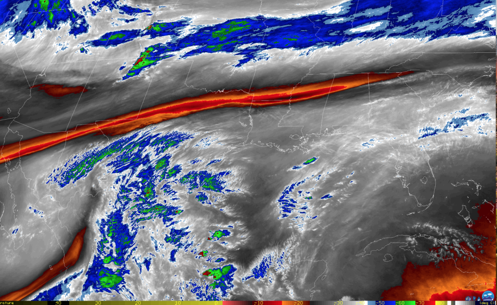
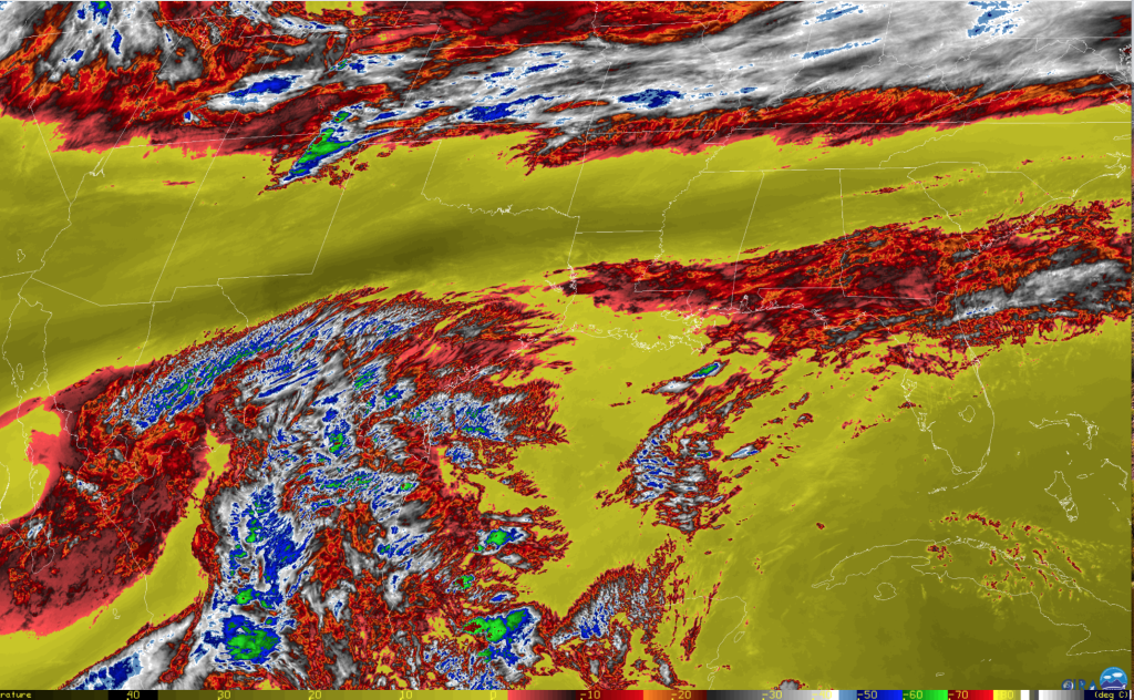
The GOES-16 water vapor imagery for all 3 channels showed a narrow band of very warm brightness temperatures (implying sinking air and a dry atmosphere) on Friday morning (1502 UTC) 9 Feb 2018.
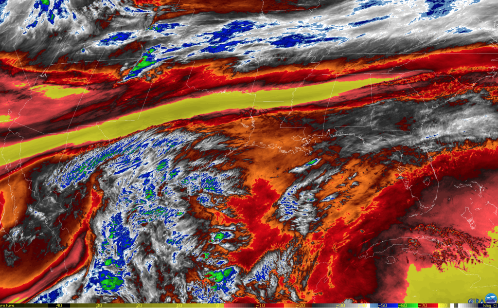
GOES-16 6.9 micron (“mid-level”) water vapor image at 1502 UTC/9 Feb 2018.
GOES-16 6.2 micron water vapor image (“high level”) at 1502 UTC/9 Feb 2018.
GOES-16 7.3 micron water vapor image (“low level”) at 1502 UTC/9 Feb 2018.
This narrow zone of sinking air is on the southern (anticyclonic) side of a very strong upper level jet draped across the CONUS, seen in the 1200 UTC 300 mb analysis below. The dry slot stretches back into the Pacific south of the CONUS jet.
 Notice how the brightness temperatures within the narrow zone are quite distinct, being at the very warm end of the scale (for this time of year). So does seeing these warm brightness temperatures at all 3 water vapor channels indicate a lack of moisture through the column. Well, not necessarily. Check out the surface plots below at 1200 UTC and 1500 UTC on 9 Feb, with corresponding GeoColor imagery for these same times. Bluish clouds in the GeoColor imagery indicate water clouds, which goes along with the low overcast conditions shown in the METAR plot. By 1500 UTC the GeoColor nighttime imagery has morphed into visible imagery, verifying the low clouds streaming north from the Gulf of Mexico. GeoColor imagery is not currently a baseline product, but CIRA can provide it to your WFO if you would like to try it.
Surface (METAR) plot at 12 UTC on 9 Feb 2018. Note the overcast conditions extending across northeast TX into southeast OK.
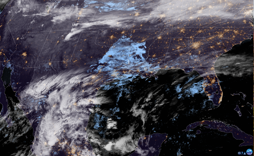
GOES-16 GeoColor image at 1202 UTC on 9 Feb. Lower level (water) clouds are bluish, while ice clouds are white. City lights are shown during nighttime imagery.
Surface (METAR) plot at 15 UTC on 9 Feb 2018.
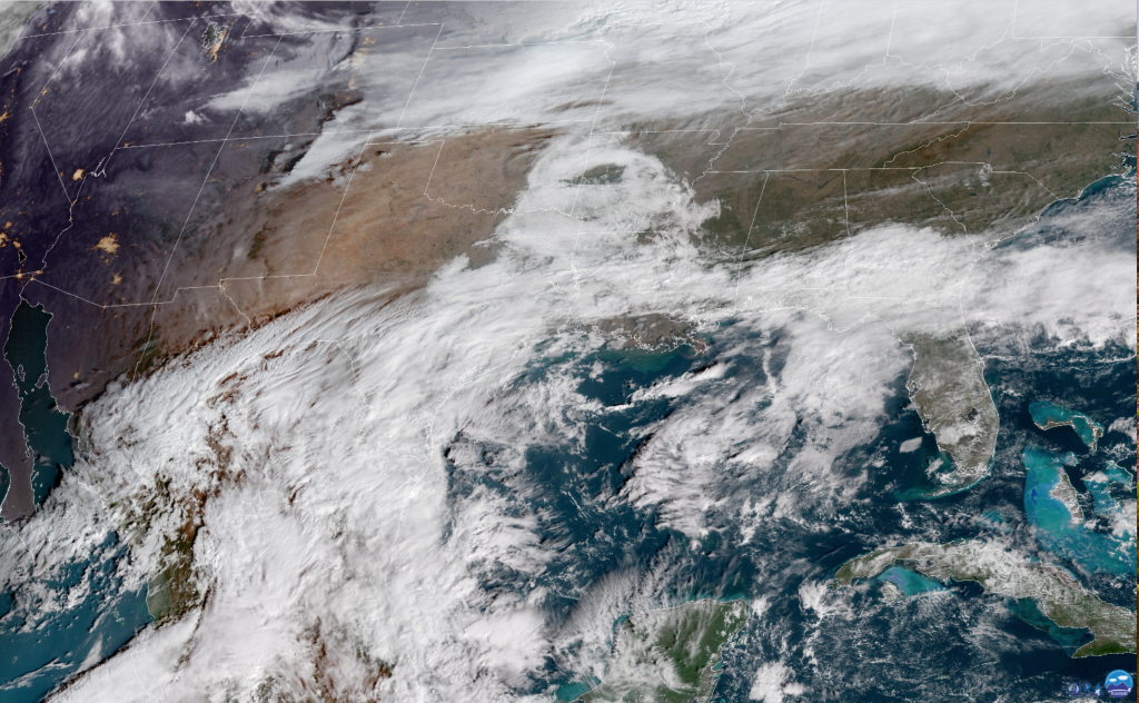
GeoColor image at 1502 UTC 9 Feb.
The satellite imagery and METAR plots indicate relatively deep low level moisture that extends northwards across a portion of the very warm/dry slot shown in the water vapor imagery. The 1200 UTC 9 Feb sounding from Dallas (DFW) in northeastern TX confirms the low level moisture (note that DFW at 1200 UTC reported scattered clouds at 1800 ft (AGL) and a 3000 ft solid cloud deck).
Dallas sounding at 1200 UTC on 9 Feb.
The moist layer extends from the surface to just above 900 mb. Why is it that this moisture is not detected by the water vapor bands, even the lowest one? The answer lies in what the weighting functions look like for the different water vapor channels for this sounding. You can see what these look like on the real-time CIMSS site at https://cimss.ssec.wisc.edu/goes/wf
For the Dallas sounding shown above the weighting functions are shown in the plot below for the 3 water vapor channels.
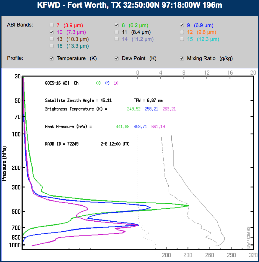
The high level water vapor channel has a single weighting function peak around 400 mb, while the other two channels have a dual peak. Even though the sounding showed that conditions were quite dry above the low level moist layer, there is just enough moisture to saturate the other two channels before reaching this low level moist layer aob 900 mb. The low-level water vapor image (7.3 micron band) appears to have a small contribution nearly to the surface, and indeed, if you look closely at that image (above) you do see a slight difference in the color within the warm/dry band in northeastern Texas. But for the most part the main message from the water vapor imagery would be a lack of moisture, yet clearly there is a low-level saturated layer. This case indicates that interpreting water vapor imagery in regards to the amount of moisture present is not straightforward. An earlier blog (go here to see the blog) showed an even more extreme case near San Diego using GOES-15 Sounder imagery (basically the same 3 water vapor channels that are on GOES-16, but at far worse horizontal resolution (10-km; and temporal resolution of course). In the San Diego case all 3 channels suggested dry conditions, but in fact the San Diego sounding had a record level of Precipitable Water (PW) for the time of year, but the moisture, while deeper than in this case, was all present below where the 3 channels saturated. This again could be seen using the weighting function profiles.
Bottom line – caution must be used when inferring a moisture profile using water vapor imagery, and the imagery does not indicate the actual value of moisture that may be present. So is there a to determine how much moisture is present in the atmosphere (besides the raob)? Indeed there is such a product, known as the Advected Layered Precipitable Water (ALPW) product. The ALPW product uses data from Polar orbiting satellites that have instrumentation that detects the amount of moisture (PW) in the atmosphere, with the ability to also see through clouds (which saturate water vapor imagery, unless of course we have a case like this one where the channels saturate before reaching the level of the clouds). The advantage of looking at the ALPW product versus looking at ABI water vapor bands is that it provides a quantitative value for the moisture in a given layer without the need to think about weighting function profiles or other complications (e.g., zenith angle) that affect your interpretation of assessing moisture from ABI water vapor bands alone. The cursor readout function on AWIPS can be used with the ALPW imagery to get read-outs of the PW values for each layer. Forecasters are familiar with the Total PW product on AWIPS, but more recently CIRA has developed the ALPW product, which is an “advected” version of the LPW product where the moisture present in 4 different layers is displayed. The ALPW product for 1500 UTC on 9 Feb is shown below (at times there are missing swaths in the imagery and this was the case over the area of interest at 1200 UTC, so 1500 UTC imagery is used). This image is from AWIPS2, using the 4-panel display to see each individual layer in one image. The imagery is available at 3-h intervals, and real-time imagery can be seen at http://cat.cira.colostate.edu/sport/layered/advected/lpw.htm . Training for this product is available at the VISIT site at http://rammb.cira.colostate.edu/training/visit/training_sessions/advected_layer_precipitable_water_product/
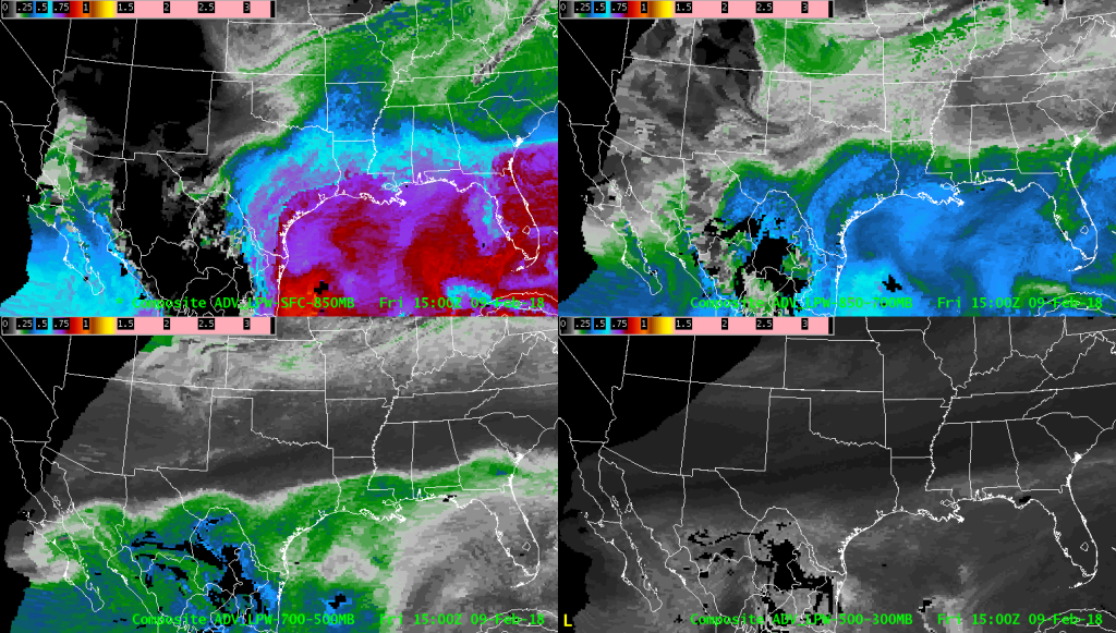 The ALPW image above depicts very dry conditions in the upper two layers (aob 700 mb), consistent with the sounding at Dallas and the water vapor imagery (which had the most contribution in these layers per the weighting functions). But the ALPW does show a nice moisture plume extending north/north-northeast into northeastern Texas, southeastern Oklahoma and into Arkansas in the lowest layer (surface to 850 mb). In the next higher layer most of this moisture is just making it towards the Dallas areas. In practice, the most information can come from using the GOES-16 water vapor imagery, with its much higher time and space resolution, in concert with the ALPW imagery. The ALPW imagery is not currently an AWIPS baseline product, but if you would like to try it at your WFO contact Dan Bikos or myself and it can be delivered to AWIPS over the LDM in real-time.