JPSS (SNPP and NOAA-20)

Puttippoq? Aatsuu

Posted on February 20, 2020 by Curtis Seaman

For once, I don’t have all the answers. That’s why I said “aatsuu“. That is an Inuit (Inuktitut) word for “I don’t know.” We’re learning Inuit language today because I wonder how they would describe a recent event in Antarctica. You see, I had been told growing up that the Inuit had more than 30 different words for “snow”, so who better to describe the changing surface properties of snow and ice?

But, as it turns out, that is a controversial statement. It has led to what linguists refer to as “the Great Eskimo Vocabulary Hoax.” There are many other blogs and podcasts that have talked about this “myth“. Exactly how many Inuit words there are for snow (or ice) depends on a lot of factors. The two biggest factors are: What is an “Inuit” language? And, what is a word? “Inuit” used here is a blanket term used to describe the native people of the North American Arctic and a few groups in far-eastern Siberia, which includes distinct groups of people that call themselves Inuit, Inupiat, Yupik, and Alutiit, among others, and have a variety of different languages. One commonality is that they all have agglutinative languages. Simply put, they combine root words with modifiers to create complex words that take the place of phrases. It is summarized succinctly in this comic. So, we might describe snow as “wet and heavy” or “light and fluffy”, while an agglutinative language would say “snowwetandheavy” or “snowfluff” to mean the same thing.

If you focus only on the root words, you get a small number of words that is similar to the number of words in English. If you add in all the possible modifiers, you get a limitless number. (Some of these are amazingly specific, such as qautsaulittuq: “ice that breaks when its strength is tested using a harpoon.”)

As part of the International Polar Year 2007-2008, the Sea Ice Knowledge and Use (SIKU) project (“siku” is the Inuit root word for “ice”) combined the efforts of physical and social scientists to better characterize our collective understanding of ice behavior in the Arctic by studying the native Arctic residents’ understanding of ice behavior, in part, through their culture and language. The discussion on the variety of words for snow and ice takes up five chapters of this compilation of SIKU research. That’s where I learned that puttippoq means an ice surface that has become wet due to melting. (You can read their take on the Great Eskimo Vocabulary Hoax here.)

Didn’t think you’d see a discussion on linguistics in a blog about satellite meteorology, did you? So, let’s get to the satellite meteorology. We’ll start with a look at what I previously called the “mystery channel“, although a better name for it is the “snow band”, since it is very sensitive to the properties of snow and ice.

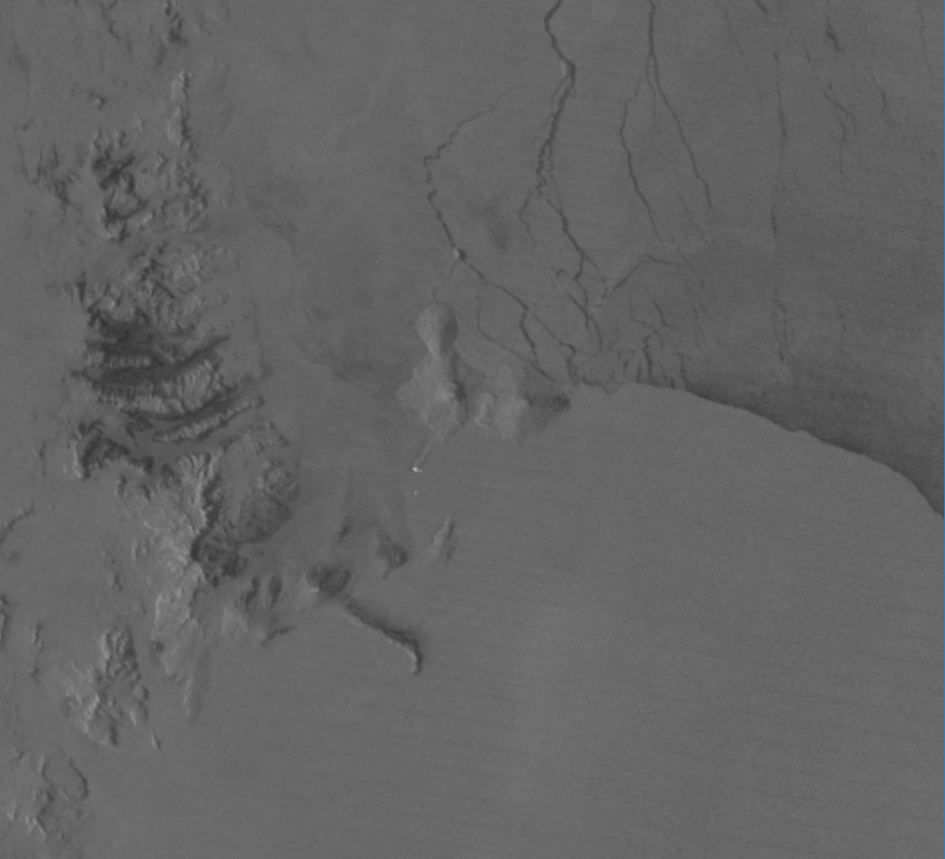
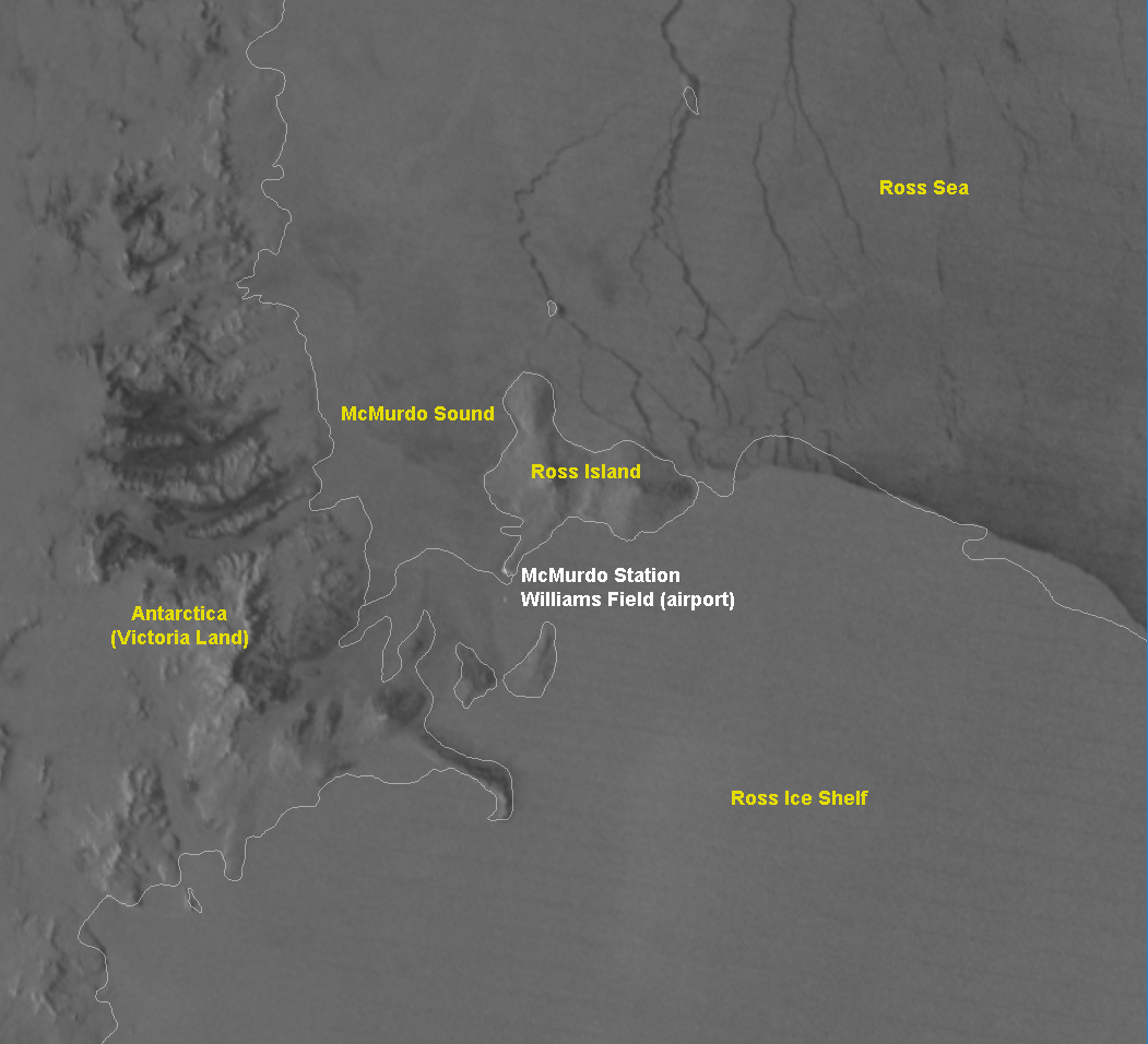
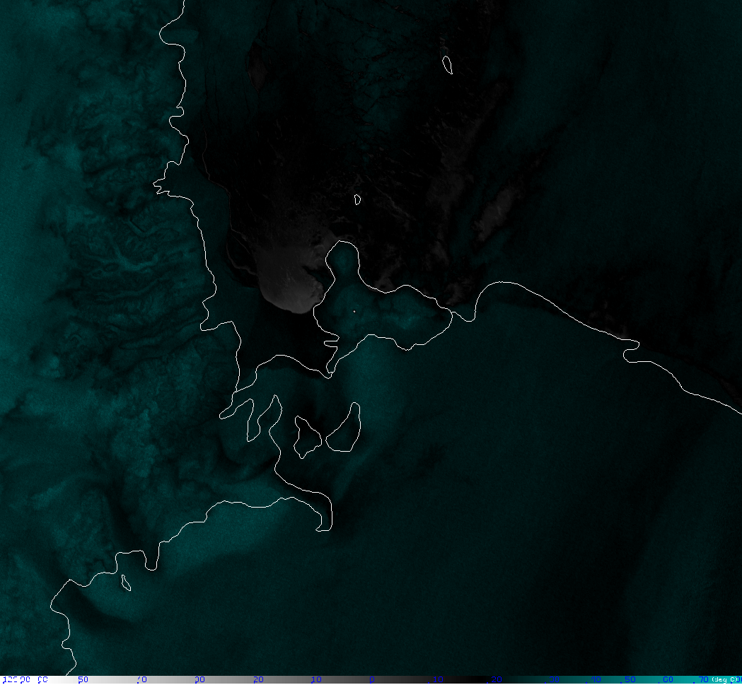
As always, it is best to view this video in full screen mode. What you are seeing is a compilation of VIIRS band M-08 (1.24 µm) images from both S-NPP and NOAA-20 from 12-13 February 2020, and there are two interesting things to note. First, the left half of the image is the high-elevation Antarctic Plateau, which contains a very bright feature that is very stationary. The right side of the image is low-elevation and contains the southernmost tip of the Ross Ice Shelf (outlined on the map). The Transantarctic Mountains (or, more specifically, the Queen Maud Mountains) in the middle separate the two regions. Pay attention to the expanding dark region on top of the ice shelf.

Since it is difficult to focus on more than one thing at a time, let’s focus on the ice shelf first. (Coincidentally, I haven’t found an Inuit word for “ice shelf”, but I did find sikuiuitsoq, which means “ice that doesn’t melt” – used to refer to ice that has been around a long time, which certainly applies to the Ross Ice Shelf.)

Animation of VIIRS M-08 images (12-13 February 2020)

This is an animated GIF that you will have to click to view. This feature shows up in the longer-wavelength bands, M-10 (1.61 µm) and M-11 (2.25 µm):

Animation of VIIRS M-10 images (12-13 February 2020)

Animation of VIIRS M-11 images (12-13 February 2020)

But, see if you can find it in the shorter-wavelength bands, M-07 (0.86 µm) and M-05 (0.67 µm):

Animation of VIIRS M-07 images (12-13 February 2020)

Animation of VIIRS M-05 images (12-13 February 2020)

At the shorter wavelengths, the feature only appears at certain times, suggesting a viewing angle dependence on the reflectance. That means the bidirectional reflectance distribution function (BRDF) is not uniform.

The explanation for this feature is pretty simple. The cold air over the Antarctic Plateau sinks down through the canyons in the Queen Maud Mountains, and as it descends, the air compresses and warms. These are called katabatic winds. In this case, the katabatic winds are aided by the synoptic scale flow as evidenced by the cloud motion. This relatively warm wind is likely melting the top surface of the Ross Ice Sheet, causing a drop in reflectance in the short-wave infrared (IR) similar to what we’ve seen before. In fact, the darkest regions of those canyons are where the howling katabatic winds have scoured away all the snow, leaving behind only the oldest glacial ice. And glacial ice has the largest grain sizes of any of the ice out there, which we know is a big factor on ice reflectivity in the shortwave-IR. (Watch those animations again and note that M-11 appears to provide the strongest signal of blowing snow coming out of those canyons. This is exploited by the Day Snow/Fog RGB.)

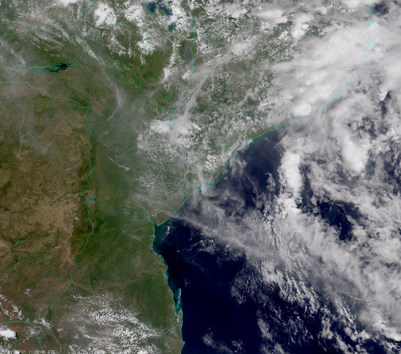
For comparison purposes, let’s look at the Natural Color RGB (also known as the Day Land Cloud RGB), made up of M-05 (blue), M-07 (green) and M-10 (red):

Animation of VIIRS Natural Color RGB composite of M-5, M-7, and M-10 (12-13 February 2020)

And, what we are calling the VIIRS “Snowmelt” RGB (M-05/blue, M-08/green, M-10/red):

Animation of VIIRS Snowmelt RGB images (12-13 February 2020)

And, finally, a variation of the “Snow” RGB developed by Météo-France (M-11/blue, M-08/green, M-07/red):

Animation of VIIRS MeteoFrance Snow RGB images (12-13 February 2020)

The inclusion of M-08 makes a big difference on the visibility of this feature. And, in contrast, this is one application where True Color imagery (M-03/0.48 µm/blue, M-04/0.55 µm/green, M-05/0.67 µm/red) is of no help at all:

Animation of VIIRS True Color images (12-13 February 2020)

As for the second region of interest from the original video, “Aatsuu”. We have a region of ice and/or snow in the Antarctic Plateau that is significantly brighter than its surroundings in the shortwave IR. The question is: why is it such a well-defined shape with a distinct edge to it? Here are all the same bands and RGBs as above:

Animation of VIIRS M-05 images (12-13 February 2020)

Animation of VIIRS M-07 images (12-13 February 2020)

Animation of VIIRS M-08 images (12-13 February 2020)

Animation of VIIRS M-10 images (12-13 February 2020)

Animation of VIIRS M-11 images (12-13 February 2020)

Animation of VIIRS True Color RGB images (12-13 February 2020)

Animation of VIIRS Natural Color RGB images (12-13 February 2020)

Animation of VIIRS Snowmelt RGB images (12-13 February 2020)

Animation of VIIRS MeteoFrance Snow RGB images (12-13 February 2020)

We know that smaller particle size leads to increased reflectivity in the shortwave IR. And, fresh snow typically fits that bill. But, fresh snow tends to appear more streaky (technical term) in satellite images. It’s the distinct edges that are so puzzling.

Anyone with more experience about the ice properties on the Antarctic Plateau out there? Or, experts at what makes snow and ice bright in the shortwave IR? If so, feel free to post a comment. (But, any theories involving UUSOs or UUIOs [Unidentified Under Ice Objects] will be placed in this blog’s trash.)

If not, isn’t this what graduate students are for?

Remote Islands VI: Return to Gough

Posted on February 4, 2020 by Curtis Seaman

You youngins are not old enough to remember, but we took a look at Gough Island before. Well, not directly, but as part of the British territory of Saint Helena, Ascension and Tristan da Cunha eight years ago. We also did a special feature on Saint Helena and Ascension four years ago. So, why are we re-visiting a group of tiny islands in the middle of the South Atlantic Ocean for a third time? Because of the great view that VIIRS provided earlier this month, and because Gough Island is an interesting place.

For starters, it rhymes with “scoff” and not with “dough” despite the spelling. So now you know. It is also home to one of the more unique jobs in meteorology. It has no permanent residents, but every year a group of 5-10 people are brought in to run the weather station on it for the South African Weather Service and study the biology of the island for the South African National Antarctic Programme (SANAP) even though it is a British island. (At least one member of the team has to be a doctor, since there are no hospitals within 400 km and boats only stop by a couple of times per year.) From the pictures and video, it certainly looks like unique place to spend a year.

Now, on to the interesting satellite imagery. We begin our visit to Gough Island with a loop from Meteosat-11, and its imager, SEVIRI (PDF document):

Note that Meteosat data was provided to NOAA by EUMETSAT and the video above shows their “Enhanced” Natural Color RGB. I can also take this opportunity to promote the fact that we are now allowed to share Meteosat imagery on our ultra-popular website, SLIDER, which is where the above loop came from.

Credits and advertising out of the way, did you see Gough Island? If not, you could try viewing the video in full-screen mode. Or, it might help if I zoomed in on the area, like this:

Meteosat-11 “Enhanced” Natural Color RGB (07-18 UTC, 5 January 2020)

The southernmost green dot is Gough Island. The other green dots are Tristan da Cunha, Inaccessible Island, and Nightingale Island. What caught my attention was two things: it’s rare to get such a clear view of these islands and the waves produced by Gough Island clearly impact clouds that never even passed over the island. Of course, having come from SEVIRI, this loop is limited to 3 km resolution (since the HRV band isn’t part of this RGB, and doesn’t normally cover this part of the world).

What if we had 375 m resolution? What would that look like? Well, on VIIRS, it looks like this:

NOAA-20 VIIRS Natural Color RGB composite of channels I-01, I-2 and I-3 (14:38 UTC 5 January 2020)

Click on the image to view the full resolution. It’s worth it.

It should be noted that I haven’t applied the same “enhanced” version of the Natural Color RGB that removes the cyan color of ice clouds and snow. Another difference is something that you don’t see in the SEVIRI loop: sun glint. That’s because Meteosat-11 isn’t viewing the scene from the same angle as VIIRS.

Look closely downwind (or leeward) of Gough Island and you’ll see from the sun glint that the island is producing waves not only in the atmosphere, but on the surface of the ocean:

Same image as above, only zoomed in on Gough Island

Of course, if you clicked on the sun glint link, you saw a more extreme example of this, and if you bothered to read the article, you also saw the explanation (written much more succinctly and accurately than I could without plagiarism).

That was only the NOAA-20 view. We also have the Suomi-NPP view, which covered this area before and after NOAA-20. Here are all three views combined:

Animation of VIIRS Natural Color RGB images (5 January 2020)

You have to click on the image above to see the animation play. Now you can see the motion of the clouds, yet the waves are nearly stationary. That’s because they are “tied” to the island that is producing them. This is an example of trapped lee waves. And pilots beware: as this case shows, these waves are present even where there are no clouds to reveal them.

What is perhaps more interesting is that the waves in the ocean show up in the mid-wave infrared (IR) thanks to the sun glint:

S-NPP VIIRS I-04 image (13:46 UTC, 5 January 2020)

This is I-04, the 375 m resolution channel at 3.7 µm, from the first S-NPP overpass (13:46 UTC, 5 January 2020). See the waves on the lee of both Gough Island and Tristan da Cunha? (Tristan da Cunha’s waves aren’t apparent in the clouds. Since these are trapped lee waves, they are occurring below the height of the cirrus clouds to the northwest.) Now, let’s animate the three overpasses:

Animation of VIIRS I-04 images (5 January 2020)

The impact of sun glint on the these images, especially the middle one (NOAA-20) is obvious. The last image from S-NPP (15:29 UTC) has no sun glint, so these waves are much harder to spot.

Now check out the high-resolution longwave IR (LWIR) band, I-05 (11.4 µm):

Animation of VIIRS I-05 images (5 January 2020)

Pay attention to the change in scaling as revealed by the color table. Three things stand out: with this combination of scaling and color table, you can see structure in the sea surface temperature, the waves downwind of Gough are still visible in the ocean even in the LWIR, and “limb cooling” is something to watch out for.

More detail on the items of note: the sea surface temperature (SST) structure is easier to spot in I-05 because it is not impacted by sun glint. This is because the Earth emits significantly more radiation in the LWIR than what it receives from the sun. In the midwave-IR, the contribution from the sun is significant (as these images show). The waves are still visible in I-05 because the winds on the downward portion of the wave are hitting the ocean surface and modifying the exchange of heat between the atmosphere and the ocean, leading to waves of warmer and cooler SST. And, third, “limb cooling” is the name given to the fact that, at high satellite viewing angles, the path length of the radiation through the atmosphere increases, and more radiation comes from higher up where temperatures are colder. (More on limb cooling may be found on slides 19-21 here.) Look to the clear sky areas on the left edge of the swath on the first I-05 image and compare it to the middle image. Then do the same for the right edge of the swath on the last image. The limb cooling effect is readily apparent.

There’s one more interesting thing from this same scene. Look at the True Color images from these three overpasses:

Animation of VIIRS True Color RGB images (5 January 2020)

See any variations in the color of the ocean not related to sun glint? That is phytoplankton, a source of life and death in the ocean. In fact, Gough Island’s location, where warmer sub-tropical water mingles with colder mid-latitude water is what makes it such a great nesting site for birds. The fish eat the phytoplankton and the birds eat the fish. Unfortunately, stowaway mice brought to Gough Island by accident are eating the birds.

All that interesting science from one tiny island in the middle of the South Atlantic Ocean.

Posted in Uncategorized | Tagged Atlantic, false color, Gough Island, I-1, I-2, I-3, I-4, I-5, M-3, M-4, M-5, remote island, resolution, RGB composite, true color | Comments Off

The east coast of Australia is on fire!

Posted on November 18, 2019 by Curtis Seaman

There’s an ongoing serious situation in Australia: the bush in New South Wales and Queensland is on fire.

Here’s a look at what the Advanced Himawari Imager (AHI) on Himawari-8 saw on 8 November 2019: click here.

What you see in that loop is the “Natural Fire Color RGB” (known to American forecasters as the “Day Land Cloud Fire RGB”) on the left (link to PDF description here), and the “Fire Temperature RGB” on the right (link to PDF description here). These are precisely the products we debuted on this blog seven years ago when we first looked at fires in Australia. Except, now there is a difference: the “Natural Fire Color RGB” is now made with the 3.7 µm band as the red component (replacing the 2.25 µm band I used originally), since the 3.7 µm channel is even better at detecting fires. This also means that we can produce the VIIRS version using “I-band” resolution (375 m). AHI, used in the loop I linked to above, has 2 km resolution* for the mid- and shortwave infrared (IR) bands.

Along the coast, near the northern edge of the images is Brisbane, the third largest city in Australia. Near the southern edge of those images is Sydney, the largest city in Australia. As you can see from Himawari-8, much of the area between the two is on fire. And, this is not the “Outback” where very few people live. This region contains some of the highest population density in Australia, and it’s also prime habitat for koalas, which don’t live anywhere outside of eastern Australia (except in zoos).

It’s no secret that resolution plays in big role in fire detection from satellites. We’ve covered this many times before. But, to hammer the point home (bit of American slang), here’s the resolution difference between VIIRS and AHI in full view from 3:50 UTC on 7 November 2019:

Himawari-8 AHI Day Land Cloud Fire RGB composite of bands 2, 4, and 7 (03:50 UTC, 7 November 2019)

S-NPP VIIRS Day Land Cloud Fire RGB composite of bands I-1, I-2 and I-4 (03:49 UTC, 7 November 2019)

As always, click on each image to bring up the full resolution version. If you just look at the elephant-thumbnail-sized images above without clicking on them, you might get the impression that fires are easier to spot with AHI than with VIIRS. That’s because AHI makes it appear that the entire 2km-wide pixel* is full of fire, when a fire typically only fills a very small percentage of the total area of the pixel. With 375 m resolution**, VIIRS more accurately pinpoints the locations of fire activity. Although, it should be noted that even this is still a larger scale than most fire fronts. To be really accurate, you need something with the resolution of Landsat’s OLI, or a similar radiometer attached to an aircraft – except these high-resolution instruments don’t provide full global coverage multiple times daily like VIIRS, or hemispheric coverage every 10 minutes like AHI. (*On AHI [and ABI and AMI] pixels may be approximated as square-shaped solid angles that are projected onto the curved surface of the Earth from a point roughly 36,000 km above the Equator. 2 km is the width of an IR pixel at the sub-satellite point [on the Equator], where the resolutions are the highest. **VIIRS pixel resolutions vary across the swath by a factor of 2 between nadir and edge of scan, as we shall see. 375 m is the nadir value.)

For completeness, we can do the same comparison with the Fire Temperature RGB:

Himawari-8 AHI Fire Temperature RGB composite of bands 5, 6 and 7 (03:50 UTC, 7 November 2019)

S-NPP VIIRS Fire Temperature RGB composite of bands M-10, M-11 and M-12 (03:46 UTC, 7 November 2019)

This time, we’re comparing 2 km resolution (AHI) against 750 m resolution (VIIRS), so the differences aren’t as stark. But, this is a good opportunity to remind everyone that the Fire Temperature RGB provides information on fire intensity, while the Natural Fire Color (Day Land Cloud Fire) RGB provides information on fire detections (plus smoke and burn scars), and should be used more as a “fire mask”.

There’s another resolution difference that is easy to see from these fires, and it can be quite significant. I first noticed it when looking at this animation I made of the VIIRS Fire Temperature RGB from 1-11 November 2019:

Animated GIF of VIIRS Fire Temperature RGB images (1-11 November 2019)

You have to click on the animation to get it to play.

Did you notice the same thing I did? You probably noticed the explosive growth of the fires from 7-9 November, but that’s not what I’m talking about. (Hint: Pay close attention to the nighttime images.) At night, without any sunlight present, you lose information on clouds and the background land surface, and only the fires are visible (unless they are obscured by clouds). That’s where today’s feature of interest resides. I’ll zoom in on some of the fires from 5 November 2019 to make it easier to see:

Animated GIF of VIIRS Fire Temperature RGB images (5 November 2019)

The image from 14:01 UTC comes from S-NPP, while the image from 14:52 comes from NOAA-20. Is NOAA-20 better than S-NPP at detecting the fires? Well, the reverse happened two nights later:

Animated GIF of VIIRS Fire Temperature RGB images (7 November 2019)

This time, the fires appear hotter (brighter) in the 15:03 UTC image, which came from S-NPP. The 14:12 UTC image came from NOAA-20. Here’s a sequence of three images from 10 November where the NOAA-20 image is sandwiched by two S-NPP images:

Animated GIF of VIIRS Fire Temperature RGB images (10 November 2019)

So, why do the fires appear brighter in some images and not others? It’s possible that the fires are becoming more active in the middle image (due to an increase in winds, for example), but it’s more likely that you are seeing the direct result of resolution differences between the various overpasses. “But, I thought both VIIRS instruments had the same resolution,” you might say as though it were a question. And that statement would suggest that you forgot about the “bowtie-effect”. (Not the effect that has anything to do with diamonds, but the effect I wrote a whole chapter about here [PDF].) If you read the **above you would already know that the resolution of VIIRS degrades by a factor of two between nadir and the edge of scan. And, if you didn’t already know, NOAA-20 and S-NPP are positioned in space a half-orbit apart. This means that, in the time it takes between a NOAA-20 overpass and a S-NPP overpass, the Earth has rotated by half the width of the swath (approximately). So, when one VIIRS instrument views something at nadir, it will be close to the edge of scan on the other satellite (and have more coarse resolution as a result).

So, in the last animation, the first image (14:05 UTC) is S-NPP viewing the fires from the east near the edge of scan, the middle image (14:56 UTC) is NOAA-20 viewing the fires near nadir, and the third image is S-NPP viewing the fires from the west – even closer to the edge of scan. (Plus, the terrain is sloping away from S-NPP in the last image as well.)

Those factors contribute to the changing appearance of the fires. They also highlight the value of having two VIIRS instruments in space: if one satellite doesn’t get a good look at a fire, the other one likely will.

By the way, these fires have been producing a lot of smoke. Here is a loop of VIIRS True Color images from 6-11 November:

And the view from the ground is even more apocalyptic:

https://twitter.com/LunnKel/status/1194403173303083008

https://twitter.com/bangtanxzia/status/1194191340856152065

Posted in Uncategorized | Tagged Australia, false color, fire, Fire Temperature RGB, Himawari, Natural Fire Color RGB, RGB composite, true color | 3 Comments

Polar Opposites

Posted on August 15, 2019 by Curtis Seaman

As we all know, the furthest south you can travel is to the South Pole – the Geographic South Pole, not the Magnetic South Pole or the Geomagnetic South Pole. When you get there, try to face east if you can. (This is easier to do at the “Ceremonial South Pole” than it is at the actual South Pole.)

The furthest south you can get by boat is an island off the coast* of Antarctica, called Ross Island. (*The term “coast” is used loosely here, since Ross Island is usually connected to Antarctica by the Ross Ice Shelf.) At the southern tip of Ross Island is the largest “city” in Antarctica: McMurdo Station. McMurdo is the port-of-entry for most visitors to Antarctica. It is also home to a ground station that receives data from NOAA-20 (and many other satellites). So, if you love the lower latency that comes with NOAA-20 VIIRS data, you have McMurdo Station to thank. (S-NPP data is only downlinked at Svalbard – once per orbit – while NOAA-20 is downlinked at both Svalbard and McMurdo.) This is the location of today’s resolved mystery.

The mystery began with the development of a new website for viewing global VIIRS imagery: Polar SLIDER*. (*Shameless self-promotion: I helped develop that website.) If you click on that link, choose “Southern Hemisphere” from the Sector menu to view Antarctica. With every product, you can zoom in anywhere on the globe* to view the full resolution data. (*Claim is void near the Equator.) Under the Product menu, you can choose between all 22 VIIRS channels (16 M-bands, 5 I-bands, and the Day/Night Band), or from a list of imagery products and cloud products. (And we are always working to add new products.) Since it’s perpetual night down there right now, you’ll notice that the visible and near-IR bands don’t give you much information – except the Day/Night Band, of course, which can provide images like this:

NOAA-20 VIIRS DNB image (14:25 UTC, 14 August 2019)

Ross Island is in the center of that image. That bright light at the southern tip of Ross Island is McMurdo Station. The second bright light south of that is the “airport“. Here’s an annotated image with the map plotted on it:

NOAA-20 VIIRS DNB image of Ross Island and surroundings (14:25 UTC, 14 August 2019)

As always, click on an image to see it in full resolution. Now that we have our bearings, let’s look at the high resolution mid-wave IR band (I-4/3.74 µm):

NOAA-20 VIIRS channel I-4 (14:25 UTC, 14 August 2019)

See that white dot in the middle of Ross Island? What is that? (Hint: it’s not part of the map.)

To make some sense of this, look at the color table plotted on the bottom of the image. White pixels on this scale (not counting the map) are +100°C (+373 K). In contrast, the dark turquoise color surrounding it is in the -25°C to -30°C range (243-248 K). What could be over 100°C in Antarctica in the winter? Did something catch on fire?

It turns out, it is a semi-permanent feature according to this animation collected from Polar SLIDER. (You have to click on the animation to see it play.)

Animation of VIIRS channel I-4 images (13 August 2019)

Looking at Day/Night Band images over the same time period, it also shows up as a bright spot:

Animation of VIIRS DNB images (13 August 2019)

Maybe it’s a nuclear reactor that powers all of McMurdo Station? (Nope. There was a nuclear power plant, but that was de-commissioned in 1972.) Maybe the fact that this bright (in the DNB), hot spot (mid-IR) is on top of a mountain has something to do with it? (Bingo!)

Ross Island is made up of volcanoes, the most prominent of which are Mt. Erebus and Mt. Terror (named for the ships on the original expedition that discovered them). Mt. Terror (the one on the right) is inactive. Mt. Erebus, on the other (left) hand, is the southernmost active volcano in the world. And, what’s relevant here is the fact that it is home to one of only five known lava lakes in the world. So, molten-hot liquid rock exists in an ice-covered environment where temperatures regularly dip down to -50°C or -60°C. And, it’s right next to the largest settlement in Antarctica. Sleep tight. (Since we’re less than a week away from the first sunrise of the spring, get your sleep while you can down there!)

Posted in Uncategorized | Tagged antarctica, day/night band, I-4, volcano | Comments Off

Tropical Cyclone Idai: Before, During and After

Posted on March 28, 2019 by Curtis Seaman

As of the time of this writing, there is currently a humanitarian crisis in Mozambique caused by what was Tropical Cyclone Idai. Here’s the situation as of 25 March 2019.

Wikipedia actually has a pretty detailed history of Idai. Long story short, one of the worst (“worst” meaning large negative impact on humans) tropical cyclones in recorded history for the Southern Hemisphere formed just off the coast of Mozambique on 4 March 2019. It quickly headed inland as a tropical storm, where it dropped heavy rains on northern Mozambique and Malawi. Then, it turned back into the Mozambique Channel, headed for Madagascar, stopped, turned around, rapidly intensified, and then hit Mozambique a second time as a Category 2 cyclone. After making it on land a second time, it stalled out and dissipated, dropping more heavy rain in the process on central Mozambique and eastern Zimbabwe. Here is a long loop from Meteosat-8 showing much of the life cycle of Cyclone Idai as it appeared in the longwave infrared (IR).

Here’s a visible (True Color) loop from VIIRS that covers most of the month of March:

Animation of VIIRS True Color images from both S-NPP and NOAA-20 (1-25 March 2019)

This loop has been reduced in resolution to half of its original size to save on file size. Even with only 2-3 images per day (since we combined both S-NPP and NOAA-20 images), you can still clearly see the cyclone over Mozambique early in the loop head out to sea and then turn around and hit Mozambique again, where it dumped heavy rain for several days.

But, I want to draw your attention to several of the images in that loop: the beginning, the middle, and the end. On 1 March 2019, NOAA-20 got a pretty clear view of central Mozambique:

NOAA-20 VIIRS True Color composite image (11:32 UTC, 1 March 2019)

We’ll call this the “Before” image – and this one is full resolution (750 m). (NOTE: You have to click on it show it at full resolution.) We can also look at the Natural Color RGB (also known as the Day Land Cloud RGB and about a dozen other names), which we can make with the high resolution imagery bands I-1, I-2 and I-3:

NOAA-20 VIIRS Natural Color RGB composite image (11:32 UTC, 1 March 2019)

This is also at full resolution (375 m). (Again, only if you click on it.)

The worst of the flooding occurred with Idai’s second landfall on 14 March 2019, and both VIIRS got great views of Idai prior to landfall:

NOAA-20 Natural Color RGB composite image (10:47 UTC, 14 March 2019)

S-NPP Natural Color RGB composite image (11:38 UTC, 14 March 2019)

These images were taken ~50 min. apart. And, if you couldn’t already tell, they’re the high resolution Natural Color images. This is for two reasons: 1) who doesn’t want to see tropical cyclones at the highest resolution possible? and 2) the Natural Color RGB brings out details in the cloud structure you can’t see in True Color. As we’ve discussed before, Natural Color highlights ice clouds in a cyan color, while liquid clouds are nearly white. But, if you look closely in the above images, you will see lighter and darker cyan regions in the clouds above (or at the top of) the eyewall. This is due to differences in particle size. Larger ice particles appear more cyan, while smaller ice particles appear more white. (Of course, there is also some shadowing going on, which accounts for the darkest regions.)

Another thing to note is the first image comes from NOAA-20, which was to the east of Idai. This provides a great view of the sloped structure of the west side of the eyewall. (And, not much information on the east side of the eyewall.) The second image comes from Suomi-NPP, which was to the west of Idai, looking at the east side of the eyewall. The two satellites in tandem provide an almost 3D view of the clouds in the eyewall (separated by 50 minutes, of course).

Also, see that peninsula that is just to the west of the eyewall in the last two images? (Hint: you won’t see it unless you bring up the full resolution versions.) That’s where the city of Beira is (or was). Beira was home to half a million people, and was one of the major ports in Mozambique. It took a direct hit from the eyewall of Idai, which destroyed approximately 90% of the buildings there. Beira was also ground zero for the resulting flooding, and the pictures coming out are not pretty.

This is a good segue to talk about the images from the end of the loop. NOAA-20 captured a relatively cloud-free view of Mozambique on 25 March 2019:

NOAA-20 VIIRS True Color composite image (10:42 UTC, 25 March 2019)

NOAA-20 VIIRS Natural Color RGB composite image (10:47 UTC, 25 March 2019)

These images were collected 10 days after landfall, and the flooding is still evident. Don’t believe me? Compare these “After” images with the “Before” images shown earlier (zoomed in on Beira):

Animation comparing NOAA-20 True Color RGB composite images from 1 March 2019 and 25 March 2019

Notice the fertile, green agricultural land surrounding Beira in the “before” image that is covered by brown floodwater in the “after” image. Just like what we saw in the pictures from Beira.

But, there’s a lot flooding that is not so easy to see in the True Color that shows up better in the Natural Color RGB:

Animation comparing NOAA-20 Natural Color RGB images from 1 March 2019 and 25 March 2019

Since this VIIRS Natural Color imagery has twice the resolution of True Color, this animation is too large for WordPress to play it automatically. You have to click on it to see the animation play.

We’ve talked before about differences between True Color and Natural Color when it comes to flooding, and this example shows it quite well. You see, True Color can miss flooding, because water is pretty transparent at visible wavelengths. If the water is clear, you can see through it and, from the perspective of VIIRS, you see the ground underneath the water (as long as the water is relatively shallow). If the water is muddy, like most of this flooding, it’s easier to see (since radiation reflects off the particles in the water), but it can look the same as the mud (or bare ground) that isn’t covered by water.

Natural Color uses longer wavelengths, where water is much more absorbing, so water appears nearly black. That’s why it is typically easier to see flooding against a background of non-flooded land in Natural Color than True Color. But, the flooding around Beira is so muddy, the high reflectivity in the visible channel (which is the blue component of the RGB) starts to win out, and the floodwater appears more blue than black.

We can prove it by looking at the individual bands that make up these RGB composites. Remember to click to play the animations for the I-bands:

Comparison of NOAA-20 channel I-1 images from 1 March and 25 March 2019

Comparison of NOAA-20 VIIRS channel I-1 (0.64 µm) images from 1 March and 25 March 2019

Comparison of NOAA-20 channel I-2 images from 1 March and 25 March 2019

Comparison of NOAA-20 VIIRS channel I-2 (0.87 µm) images from 1 March and 25 March 2019

Comparison of NOAA-20 channel I-3 images from 1 March and 25 March 2019

Comparison of NOAA-20 VIIRS channel I-3 (1.61 µm) images from 1 March and 25 March 2019

Note that the flooded areas look brighter in I-1 (thanks to the dirty water) and look darker in I-2 and I-3 (because they are less sensitive to the dirt in the water and more sensitive to the water itself).

The individual M-bands that comprise the True Color RGB, shown below, have been corrected for Rayleigh scattering and scaled the same as in the True Color images above:

Comparison of NOAA-20 channel M-3 images from 1 March and 25 March 2019

Comparison of NOAA-20 VIIRS channel M-3 (0.48 µm) images from 1 March and 25 March 2019

Comparison of NOAA-20 channel M-4 images from 1 March and 25 March 2019

Comparison of NOAA-20 VIIRS channel M-4 (0.55 µm) images from 1 March and 25 March 2019

Comparison of NOAA-20 channel M-5 images from 1 March and 25 March 2019

Comparison of NOAA-20 VIIRS channel M-5 (0.67 µm) images from 1 March and 25 March 2019

It is quite difficult to detect the flooding using the visible channels (M-3, M-4, M-5 and I-1) alone. But, the flooded areas are generally brighter in the “after” images. However, the water is easy to see in the shortwave IR channels (I-2, and I-3 along with M-7 and M-10, which were not shown).

Of course, this was a very long-winded way of looking at the flooding. We could have just used the JPSS Program’s official Flood Product made with VIIRS, created by researchers at George Mason University. Here is a three day composite image (composited to reduce the impact of clouds), covering 19-22 March 2019:

NOAA-20 VIIRS Flood Detection Product using a 3-day cloud-free composite (19-22 March 2019). Image courtesy S. Li (GMU).

Red and yellow areas show where flooding is detected. Gray areas are areas that were cloudy all three days. As an interesting side note, this product is validated against the Natural Color RGB. For more on this product, click here. If you want to know how much precipitation actually fell, here is a loop provided by NASA made with observations from GPM (Global Precipitation Measurement Mission):

You get bonus points if you can read the scale below the images. But, even without a magnifying glass, you can probably guess: it’s a lot of rain!

Posted in Uncategorized | Tagged false color, flood, I-1, I-2, I-3, M-3, M-4, M-5, Madagascar, Malawi, Meteosat, Mozambique, Natural Color, resolution, RGB composite, tropical storm, true color, Zimbabwe | Comments Off

Ice, Ice, Baby

Posted on January 28, 2019 by Curtis Seaman

A winter storm moved through the Northeast U.S. over the weekend of 19-20 January 2019. This Nor’easter was a tricky one to forecast. Temperatures near the coast were expected to be near (or above) freezing. Temperatures inland were expected to be much colder. Liquid-equivalent precipitation, at least according to the GFS, was predicted to be in the 1-3 inch (25-75 mm) range the day before. This could easily convert to 1-2 feet (30-60 cm) of snow. The question on everyone’s mind: who gets the rain, who gets the snow, and who gets the “wintry mix”? The fates of ~40 million people hang in the balance. This is one of the situations that meteorologists live for!

The difference between 71°F and 74°F is virtually meaningless. The difference between 31°F and 34°F (with heavy precipitation, at least) is the difference between closing schools or staying open. It’s the difference between bringing out the plows or keeping them in the garage; paying overtime for power crews to keep the electricity flowing or just another work day; shutting down public transportation or life as usual.

Of course, the obvious follow-up question is: what is the “wintry mix” going to be? Rain mixed with snow? Sleet? Freezing rain? It doesn’t take much to change from one to the other, but there can be a big difference on the resulting impacts based on what ultimately falls from the sky.

So, what happened? Here’s an article that does a good job of explaining it. And, here are PDF files of the storm reports from National Weather Service Forecast Offices in Albany, Boston (actually in Norton, MA) and New York City (actually in Upton, NY). The synopsis: some places received ~1.5 inches (~38 mm) of rain, some places received ~11 inches (~30 cm) of snow and some places were coated in up to 0.6 inches (15 mm) of ice.

Of particular relevance here are the locations that received the ice. If you took the locations listed in the storm reports that had more than 0.1 inches (2.5 mm) of ice (at least the ones in Connecticut) and plotted them on a map, they match up quite well with this map of power outages that came from the article I linked to:

Map of power outages in Connecticut as a result of an ice storm (19-20 January 2019). Image courtesy Eversource/NBC Connecticut.

Now, compare that map with this VIIRS image from 22 January 2019 (after the clouds cleared out):

VIIRS channel I-3 image from NOAA-20, 17:09 UTC 22 January 2019

As always, you can click on the image to bring up the full resolution version. This is the high-resolution imagery band, I-3, centered at 1.6 µm from NOAA-20. Notice that very dark band stretching from northern New Jersey into northern Rhode Island? That’s where the greatest accumulation of ice was. Notice how well it matches up with the known power outages across Connecticut!

The ice-covered region appears dark at 1.6 µm because ice is very absorbing at this wavelength and, hence, it’s not very reflective. And, since it is cold, it doesn’t emit radiation at this wavelength either (at least, not in any significant amount). This is especially true for pure ice, as was observed here (particularly the second image), since there aren’t any impurities in the ice to reflect radiation back to the satellite. The absorbing nature of snow and ice compared with the reflective nature of liquid clouds is what earned this channel the nickname “Snow/Ice Band” (PDF).

At shorter wavelengths (less than ~ 1 µm), ice and snow are reflective. (Note how a coating of ice makes everything sparkle in the sunlight.) This makes it nearly impossible to tell where the ice accumulation was in True Color images:

VIIRS True Color RGB composite of channels M-3, M-4 and M-5 from NOAA-20, 17:09 UTC 22 January 2019

The Natural Color RGB (which the National Weather Service forecasters know as the Day Land Cloud RGB (PDF file)) includes the 1.6 µm band, which is what makes it useful for discriminating clouds from snow and ice. And, as expected, the region of ice accumulation does show up (although it is tempered by the highly reflective nature of snow and ice in the visible and “veggie” bands that make up the other components of the RGB):

VIIRS Natural Color RGB composite of channels, I-1, I-2 and I-3 from NOAA-20 (17:09 UTC, 22 January 2019)

Another RGB composite popular with forecasters is the Day Snow/Fog RGB (PDF file), where blue is related to the brightness temperature difference between 10.7 µm and 3.9 µm, green is the 1.6 µm reflectance, and red is the reflectance at 0.86 µm (the “veggie” band). This shows the region of ice even more clearly than the Natural Color RGB:

VIIRS Day Snow/Fog RGB composite of channels (I-5 - I-4), I-3 and I-2 from NOAA-20 (17:09 UTC, 22 January 2019)

VIIRS Day Snow/Fog RGB composite of channels (I-5 minus I-4), I-3 and I-2 from NOAA-20 (17:09 UTC, 22 January 2019)

Breaking things up into the individual components, we can see how the ice transitions from being reflective in the visible and near-infrared (near-IR) to absorbing in the shortwave-IR:

VIIRS high-resolution visible channel, I-1, from NOAA-20 (17:09 UTC, 22 January 2019)

VIIRS high-resolution visible channel, I-1 (0.64 µm), from NOAA-20 (17:09 UTC, 22 January 2019)

VIIRS high-resolution "veggie" channel, I-2, from NOAA-20 (17:09 UTC, 22 January 2019)

VIIRS high-resolution “veggie” channel, I-2 (0.86 µm), from NOAA-20 (17:09 UTC, 22 January 2019)

VIIRS channel M-8 from NOAA-20 (17:09 UTC, 22 January 2019)

VIIRS channel M-8 (1.24 µm) from NOAA-20 (17:09 UTC, 22 January 2019)

VIIRS channel M-11 from NOAA-20 (17:09 UTC, 22 January 2019)

VIIRS channel M-11 (2.25 µm) from NOAA-20 (17:09 UTC, 22 January 2019)

Of course, the 1.6 µm image was already shown, so I didn’t bother to repeat it. If you squint, you can even see a hint of the ice signature at 1.38 µm, the “Cirrus Band“, where most of the surface signal is blocked by water vapor absorption in the atmosphere:

VIIRS "cirrus" channel, M-9, from NOAA-20 (17:09 UTC 22 January 2019)

VIIRS “cirrus” channel, M-9 (1.38 µm), from NOAA-20 (17:09 UTC 22 January 2019)

If the ice had accumulated in southern New Jersey or Pennsylvania, though, it would not have shown up in this channel, since the air was too moist at this time to see all the way down to the surface. But, you can compare this image with the previous images to see why they call it the “cirrus band”, since the cirrus does show up much more clearly here.

So, mark this down as another use for VIIRS: detecting areas impacted by ice storms. And remember, even though ice storms may have a certain beauty, they are also dangerous. And, not just for the obvious reasons. This storm in particular came complete with ice missiles. So, for the love of everyone else on the road, scrape your car clean of ice before risking your life out there!

Posted in Uncategorized | Tagged Connecticut, Day Snow/Fog RGB, false color, I-1, I-2, I-3, I-4, I-5, ice and snow, M-11, M-3, M-4, M-5, M-8, M-9, Natural Color, New England, New Jersey, New York, resolution, RGB composite, Rhode Island, true color | 1 Comment

Protected: Clouds at the Edge of Space

Posted on September 19, 2018 by Curtis Seaman

Posted in Uncategorized | Tagged Alaska, clouds, day/night band, M-12, M-15, M-16, mesosphere, split window difference | Comments Off

Rivers of Ice

Posted on May 24, 2018 by Curtis Seaman

Oh, Yakutsk! It has been a long time – 2012, to be exact – since we last spoke about you. It was a different time back then, with me still referring to the Natural Color RGB as “pseudo-true color”. (Now, most National Weather Service forecasters know it as the “Day Land Cloud RGB”). VIIRS was a only a baby with less than one year on the job. Back then, the area surrounding the “Coldest City on Earth” was on fire. This time, we return to talk about ice.

You see, rivers near the Coldest City on Earth freeze during the winter, as do most rivers at high latitudes. Places like the Northwest Territories, the Yukon, Alaska and Siberia use this to their advantage. Rivers that are frozen solid can make good roads, a fact that has often been overly dramatized for TV. Transporting heavy equipment may be better done on solid ice in the winter than on squishy, swampy tundra in the summer. But, that comes with a cost: ice roads only work during the winter.

In remote places like these, with few roads, rivers are the lifeblood of transportation – acting as roads during the winter and waterways for boats during the summer. But, what about the transition period that happens each spring and fall? Every year there is a period of time where it is too icy for boats and not icy enough for trucks. Monitoring for the autumn ice-up is an important task. And, perhaps it is more important to monitor for the spring break-up of the ice, since the break up period is often associated with ice jams and flooding.

We’ve covered the autumn ice up before (on our sister blog), but VIIRS recently captured a great view of the spring break up near Yakutsk, that will be our focus today.

We will start with the astonishing video captured by VIIRS’ geostationary cousin, the Advanced Himawari Imager (AHI) on Himawari-8 from 18 May 2018:

The big river flowing south to north in the center of the frame is the Lena River. (Yakutsk is on that river just south of the easternmost bend.) The second big river along the right side of the frame is the Aldan River, which turns to the west and flows into the Lena in the center of the frame.

Now that you are oriented, take a look at that video again in full screen mode. If you look closely, you will see a snake-like section of ice flowing from the Aldan into the Lena. This is exactly the kind of thing river forecasters are supposed to be watching for during the spring!

Of course, this is a geostationary satellite, which provides good temporal resolution, but not as good spatial resolution. The video is made from 1-km resolution imagery, but we are looking at high latitudes on an oblique angle, so the resolution is more like 3-4 km here. So, how does this look from the vantage point of VIIRS, which provides similar imagery at 375 m resolution? See for yourself:

(You will have to click on the image to get the animation to play.)

Animation of VIIRS Natural Color RGB composite of channels I-1, I-2 and I-3 (18 May 2018)

This animation includes both Suomi NPP and NOAA-20 VIIRS. That gives us ~50 min. temporal resolution to go with the sub-kilometer spatial resolution. Eagle-eyed viewers can see how the resolution changes over the course of the animation, as the rivers start out near the left edge of the VIIRS swath (~750 m resolution), then on subsequent orbits, the rivers are near nadir (~375 m resolution) and then on the right edge of the swath (~750 m resolution again). In any case, this is better spatial resolution than AHI can provide at this latitude.

One thing you can do with this animation is calculate how fast the ice was moving. I estimated the leading edge of the big “ice snake” moved about 59 pixels (22.3 km at 375 m resolution) during the 3 hour, 21 minute duration of the animation. That works out to an average speed of 6.7 km/hr (3.6 knots), which doesn’t seem unreasonable. Counting up pixels also indicates our big “ice snake” is at least 65 km long, and the Aldan River is nearly 3 km wide in its lower reaches when it meets the Lena River. That is in the neighborhood of 200 km² of ice!

That much ice moving at 3 knots can do a lot of damage. Just look at what the ice on this much smaller river did to this bridge:

(Make sure you watch it all the way to the end!)

Posted in Uncategorized | Tagged AHI, false color, ice and snow, NOAA-20, resolution, RGB composite, S-NPP, Siberia | Comments Off

Don’t Eat Orange Snow

Posted on April 24, 2018 by Curtis Seaman

Roughly one month ago, social media (and, later, more conventional media) outlets were inundated with numerous reports of orange snow in eastern Europe and western Asia – reports like this one, this one and this one. Of course, it wouldn’t really be a hit with the media unless someone could claim it was “apocalyptic”. And of course, the apocalypse didn’t happen. It was simply Saharan dust picked up by high winds from an intense mid-latitude cyclone and deposited far away. We’ve seen this before with VIIRS.

These reports focused on Sochi, Russia, home of the 2014 Winter Olympics. Unfortunately, every time I looked for it in VIIRS imagery, it was cloudy in Sochi. But, the plume of Saharan dust that caused this event was clearly visible over the Mediterranean:

NOAA-20 VIIRS true color composite of channels M-3, M-4 and M-5 (10:03 UTC 25 March 2018)

This image came from our new NOAA-20 VIIRS, which, at this point, is not operational and undergoing additional testing. If you look closer, you might also notice smoke or smog over Poland in the image above (upper left corner). If you really zoom in (click on the image to get to the full resolution version), you may notice a brownish tint to the snow along the north shore of the Black Sea – where the BBC report I linked to listed additional sightings of orange snow. But, the dust-covered snow shows up more clearly in this “before and after” image courtesy of S-NPP VIIRS and the @NOAASatellites twitter account:

“Before” and “After” S-NPP VIIRS true color images from 22 March 2018 (left) and 25 March 2018 (right).

(As an aside: differences in technique used to produce these true color images are likely larger than the differences between S-NPP VIIRS and NOAA-20 VIIRS, so don’t read too much into the fact that the dust-on-snow appears more clearly in the @NOAASatellites image than in my own.)

But, dust-on-snow is not limited to areas within a few thousand kilometers of the Sahara Desert. (It is limited to areas within 40,000 km of the Sahara [in the horizontal dimension, at least], since that is roughly the circumference of the Earth – and assuming you ignore dust storms on Mars.) Dust on snow can happen anywhere you have snow within striking distance of a source of dust. Another example was captured by a new Landsat-like micro-satellite, Venµs, and its non-microsat predecessor, Sentinel-2B, Landsat’s European cousin. A more dramatic example happened last week right here in Colorado. Here is a VIIRS true color image of Colorado from S-NPP VIIRS, taken on 14 April 2018:

S-NPP VIIRS true color composite of channels M-3, M-4 and M-5 (19:45 UTC 14 April 2018)

Here are similar images from NOAA-20 and S-NPP from 18 April 2018:

NOAA-20 VIIRS true color composite of channels M-3, M-4 and M-5 (19:20 UTC 18 April 2018)

S-NPP VIIRS true color composite of channels M-3, M-4 and M-5 (20:11 UTC 18 April 2018)

The trick is to compare these two images with the image from 14 April. The other trick is to know where you’re supposed to be looking. (Hint: we’re looking at the Sangre de Cristo mountains in southern Colorado.) Here’s a “before” and “after” image overlay trick I’ve used before. (You may have to refresh the page before it will work.) Both of these images are the S-NPP VIIRS ones, for simplicity:

[beforeafter][/beforeafter]

If you slide the bar left to right, you should notice the snow is more brown in the mountains just right of center in the 18 April image. There are other areas where the snow melted between the two images, plus a couple of small clouds that add to the differences. Of course, this is only 750 m resolution. We get a better view with the 375m-resolution visible channel, I-1:

[beforeafter][/beforeafter]

We lose the color information, of course, since we are looking at a single channel, but it is obvious the snow became less reflective in the 18 April image. And, we can prove that this was a result of dust. Here are the visible, true color, Dust RGB, “Blue Light Dust” and DEBRA Dust images from S-NPP on 17 April 2018, courtesy Steve M.:

S-NPP VIIRS true color composite of channels M-3, M-4 and M-5 (20:26 UTC 17 April 2018)

S-NPP VIIRS Dust RGB image (20:26 UTC 17 April 2018)

S-NPP VIIRS Blue Light Dust image (20:26 UTC 17 April 2018)

S-NPP VIIRS DEBRA Dust image (20:26 UTC 17 April 2018)

If you are unfamiliar with them, we’ve looked at the Dust RGB, Blue Light Dust and DEBRA before, here and here. As seen in the above images, this was not a difficult to detect dust case. Even Landsat-8 captured this event, which is surprising given the narrow swath and 16-day orbit repeat cycle. (Sure, it’s higher resolution than VIIRS, but will it be overhead when you need it?)

So now we get to why dust-on-snow is important. There is a growing body of research (e.g. this paper) that shows dust-on-snow has a big impact on water resources in places like the Rocky Mountains. You see, dirty snow is less reflective than clean snow. That means it absorbs more solar radiation. This, in turn, means it heats up and melts faster, leading to earlier spring run-off. The end result is less water later in the season, which opens the door to wildfires and more severe droughts. This article that, coincidentally, was published as I was writing this, sums things up nicely. It is so important, the Center for Snow and Avalanche Studies has formed CODOS: the Colorado Dust on Snow Program, whose purpose is to monitor dust on snow and provide weekly updates.

As for why you shouldn’t eat orange snow, that should be obvious. You shouldn’t eat any snow that isn’t pure white (and even that might be risky). But, feel free to eat colorful ice, as long as you know where it came from.

Posted in Uncategorized | Tagged Black Sea, colorado, DEBRA, dust, EUMETSAT Dust, Europe, I-1, ice and snow, M-3, M-4, M-5, resolution, RGB composite, true color | 1 Comment

The Arctic, Saharan-like Gulf Coast

Posted on February 1, 2018 by Curtis Seaman

Today, we’re going to take a look at another less-covered VIIRS channel on this blog: M-9, also known as the “cirrus band”. (Disambiguation: if you’re looking for the electronic musical group “Cirrus (band)“, you’re in the wrong place.) We don’t use M-9 on this blog much because it doesn’t often provide amazing images. But, it is used for a lot of practical applications, so it is worth knowing about. We are also going to say “Hello!” to Suomi-NPP’s baby brother, NOAA-20, and welcome a new VIIRS instrument in space!

Unlike M-8, the “cirrus band” (PDF) is on nearly all of the new geostationary satellites (except Himawari). It’s also on MODIS, Landsat, and several other polar-orbiting satellite imagers. The “cirrus band” is unique in that it is highly sensitive to water vapor, but is located in the near-IR (1.38 µm) where emission from the Earth is minimal. (So, contrary to popular belief, VIIRS does have a water vapor channel. It just doesn’t behave like the typical mid-wave IR water vapor channels most people are used to.)

Electromagnetic radiation at 1.38 µm is absorbed by water vapor. But, the Earth and its atmosphere are too cold to emit much at this wavelength. (Thankfully, or we would have all melted by now.) Of course, the sun is hot enough. This means the 1.38 µm radiation coming from the sun is absorbed by water vapor in our atmosphere, and the only* radiation making its way back to VIIRS is what is reflected off of clouds above the water vapor. This makes channels centered at 1.38 µm particularly useful at identifying thin cirrus that would otherwise blend in with the background on other channels. Hence, the name “cirrus band”. (* Of course, reflection off of high clouds is not the only source, as we shall see. That’s the reason for this blog post.)

So, high clouds are white and the background is black – this is the assumption when looking at VIIRS’s cirrus band (unless you’re using a funky color table). But, take a look at this image that S-NPP VIIRS took on 17 January 2018:

S-NPP VIIRS channel M-9 (“cirrus band”) image from 18:34 UTC, 17 January 2018

On my monitor, viewing angle makes a big difference as to how bright the features appear. If you are viewing this on a laptop or tablet, your screen is much easier to adjust that than my Jumbotron if it’s hard to see. You can also move your head around and see if anyone else looks at you funny. (This is also a good way to test out a TV in the store before you buy it. Will people sitting off to the side get the same view as someone directly in front of the TV? You might want to know that if hosting a party for the big game this weekend.)

Let’s zoom in on the area in question:

S-NPP VIIRS channel M-9 image from 18:34 UTC, 17 January 2018

And, give the image maximum contrast:

S-NPP VIIRS channel M-9 image displayed with maximum contrast (18:34 UTC, 17 January 2018)

There is a feature in that image that looks awfully like the coastline of the Gulf of Mexico stretching from Louisiana to the Florida panhandle. It sure looks like you can see the Mississippi River, the Tennessee River, and all the “lakes” in eastern Texas. But, I thought water vapor was supposed to absorb all the radiation before it made it to the surface! And, this is Louisiana we’re talking about. The entire coastal region of the state is a big swamp – I mean a collection of bayous. So, there should be plenty of water vapor around.

One would expect to see all the way to the surface in high-altitude arid areas, like the Bolivian Altiplano and the upper elevations of the Atacama Desert. And, you do:

S-NPP VIIRS channel M-9 image from 18:32 UTC, 1 June 2017.

But, one does not expect to see the surface of Louisiana at 1.38 µm, since it is so close to sea level and it is one of the most humid parts of the United States. Maybe something is wrong with S-NPP VIIRS? Let’s look at our new baby, NOAA-20 VIIRS:

NOAA-20 VIIRS channel M-9 image (19:25 UTC, 17 January 2018)

And, once again, with maximum contrast:

NOAA-20 VIIRS channel M-9 image displayed with maximum contrast (19:25 UTC, 17 January 2017)

Note that NOAA-20 was launched back in November 2017, and is still undergoing post-launch testing and checkout, so it has not been declared operational just yet. But, this is a good test for the new VIIRS. It can see the same surface features S-NPP did 50 minutes earlier. And, it means that both instruments are working. So, why can we see all the way to the surface of Louisiana in the “cirrus band”? Because, the atmosphere was incredibly dry.

Here’s the sounding from Slidell, LA (on the other side of Lake Pontchartrain from New Orleans) on 12 UTC 17 January 2018. Notice the precipitable water value (“PWAT”) is 2.47, which is reported on soundings in mm. That’s just less than 0.1 inches. The nearby soundings taken at Shreveport and Lake Charles reported PWATs of 2.45 mm and 2.77 mm, respectively. Normal for this time of year is about 7 times greater! (Note that he corrected his typo.)

To put this into perspective, this was drier than the Sahara Desert was a few days later:

NOAA-20 VIIRS channel M-9 image displayed with maximum contrast (12:40 UTC, 22 January 2018)

Notice you can’t see the surface of the Sahara, indicating there was more water vapor in the air over the desert than there was over Louisiana. The only thing you can see are the cirrus clouds and other clouds that made it to the upper atmosphere. This is more typical of the “cirrus band”.

Now, back to Louisiana: the dry, Arctic airmass resulted in a number of record low temperatures. Plus, this was accompanied by snow, as seen by both S-NPP and NOAA-20:

S-NPP VIIRS True Color RGB composite of channels M-3, M-4 and M-5 (18:34 UTC 17 January 2018)

NOAA-20 VIIRS True Color composite of channels M-3, M-4 and M-5 (19:25 UTC, 17 January 2018)

Snow was reported all the way to Gulf Coast, and you can see evidence of it in the images around Houston, TX, which is pretty rare. But, wait! Why didn’t we see snow in the M-9 “cirrus band” images? Because snow is not very reflective at 1.38 µm, and it blends in with the background. To show what an interesting winter it has been, here’s a map put out by the Weather Prediction Center from 18 January 2018, showing estimated total snowfall accumulations for this winter (so far). Note that an area of Mississippi and Louisiana has had approximately the same amount of snow as most of Iowa and southern Wisconsin (and even here in Northern Colorado!). All 48 contiguous United States have received measurable snowfall!

Fun fact: you can open one of the True Color images in a new browser tab, and the other image in this tab and toggle back and forth between them. This allows you to see the clouds move, and the edges of the snowfield melt. If you have eagle eyes, you can also see that the S-NPP image is sharper on the east side of the image (close to its nadir), while the NOAA-20 image is sharper on the west side (close to its nadir). The satellites are both in the same orbit, but on opposite sides of the Earth. Since the Earth is constantly rotating underneath them, and the VIIRS swath is designed to fill all the gaps at the Equator (unlike MODIS), their ground tracks at low and mid-latitudes are separated by half the width of a VIIRS swath. Nadir for one VIIRS is near the edge of the swath of the other VIIRS. (But, not at high latitudes.) The distance from Tallahassee, Florida to Houston, Texas is a pretty good rule of thumb for the spatial distance between the two satellites when they’re over the United States. Fifty minutes is a good rule of thumb for the temporal distance between them (and this is true all over the globe).

So, for once, Louisiana was colder than the Arctic (Ocean, at least) and drier than the Sahara Desert!

Posted in Uncategorized | Tagged Gulf of Mexico, ice and snow, Louisiana, M-3, M-4, M-5, M-9, RGB composite, true color | Comments Off