
Atmospheric River event of 7-10 January, 2023
January 13th, 2023 by Dan BikosBy Sheldon Kusselson and Dan Bikos
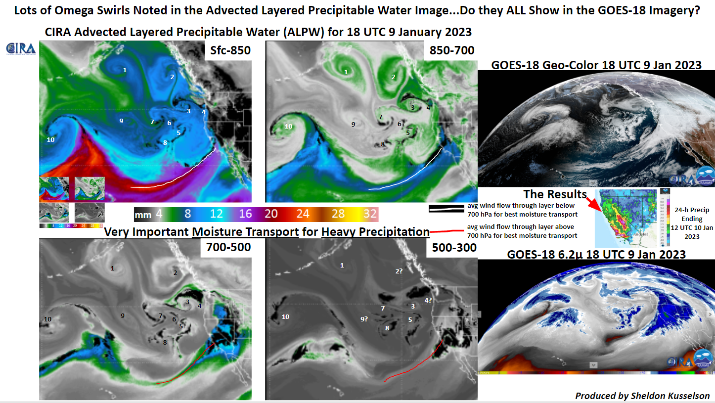
Advected Layer Precipitable Water (ALPW) Loop
Posted in: Heavy Rain and Flooding Issues, Hydrology, | Comments closed
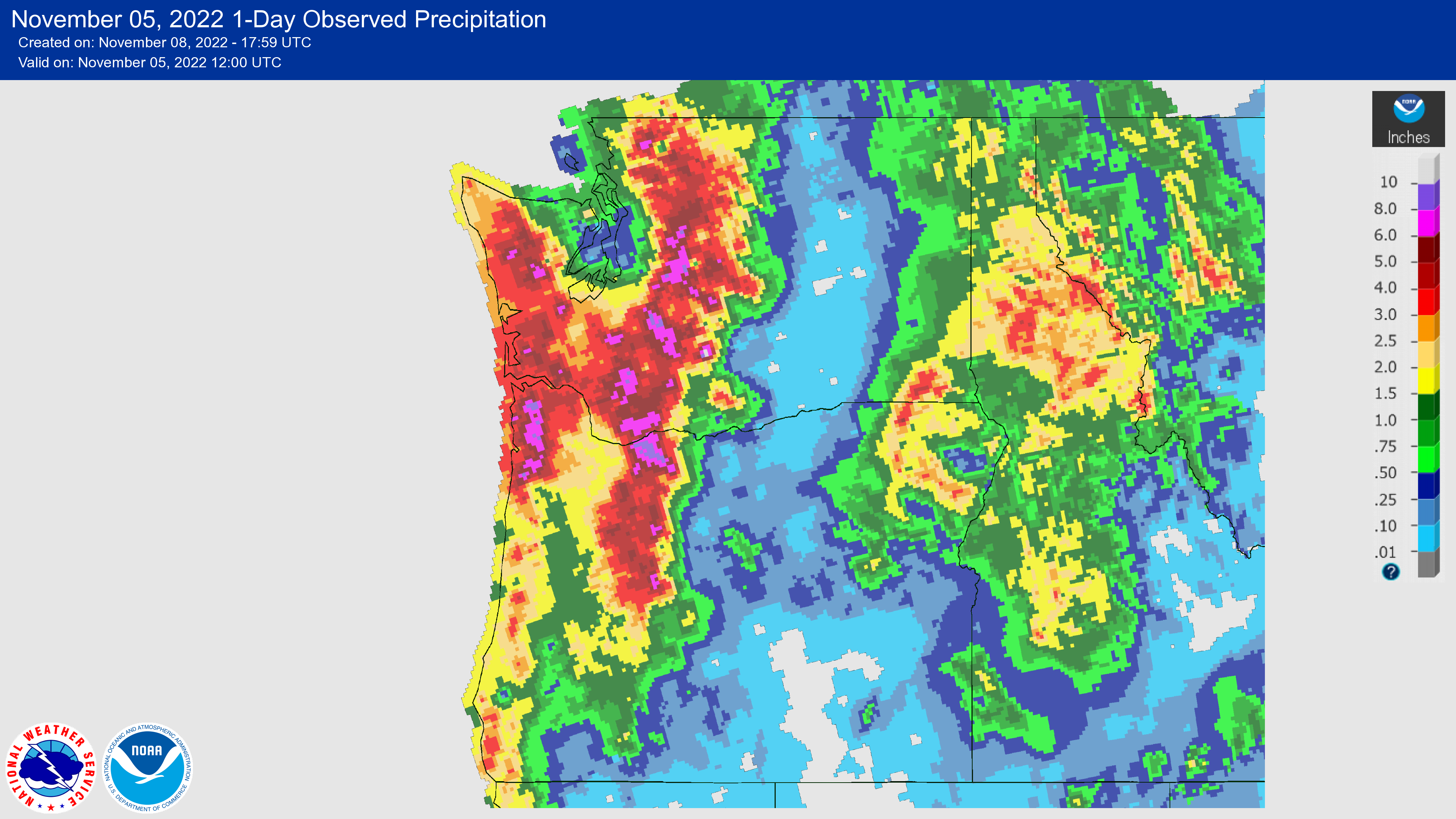
CIRA ALPW depiction of Atmospheric River of 4-5 November 2022
November 9th, 2022 by Dan BikosBy Sheldon Kusselson and Dan Bikos

Advected Layer Precipitable Water (ALPW) loop
Observed 1-Day Precipitation valid 1200 UTC 5 November 2022 over the Pacific Northwest region:
Posted in: Heavy Rain and Flooding Issues, POES, | Comments closed
Extra-tropical transition of Tropical Cyclone Fiona
September 27th, 2022 by Dan BikosBy Dan Bikos and Sheldon Kusselson
Hurricane Fiona underwent a transition from a tropical cyclone to an extra-tropical cyclone on 23-24 September 2022. The resulting extra-tropical cyclone was very intense and led to significant storm surge, wind damage and heavy rain in southeast Canada centered on Nova Scotia.
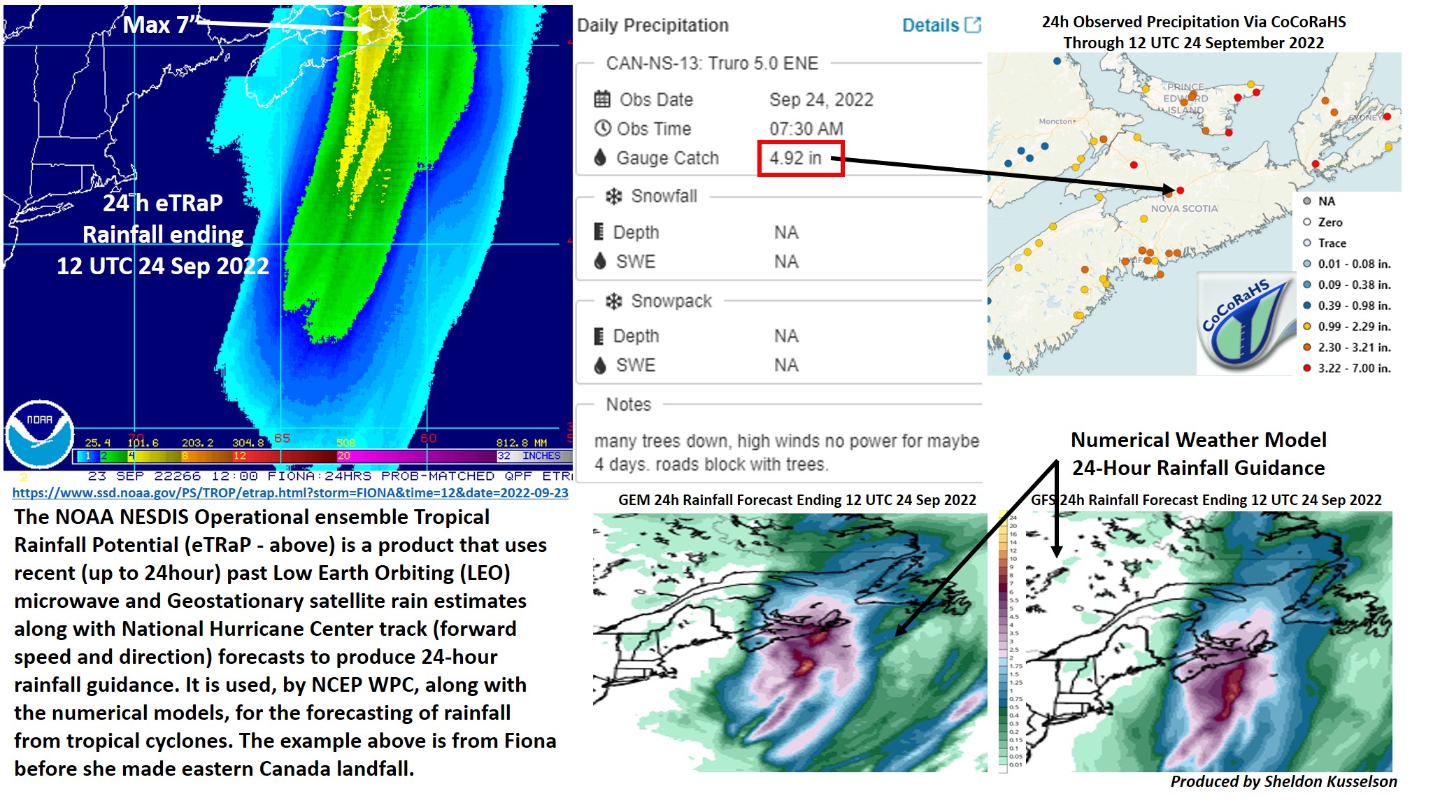
The Advected Layer Precipitable Water loop does an excellent job of capturing the transition to an extra-tropical cyclone. The lower left panel displays the precipitable water in the 700-500 mb layer. Note the dry air mass that is initially southwest of the surface low, wrap cyclonically around the low. This dry air intrusion at mid-levels is characteristic of extra-tropical cyclogenesis as the dry conveyor belt (also called dry slot) develops and intensifies. The ALPW loop also shows the abundant low-level moisture transported northward ahead of the surface low towards Nova Scotia, contributing to the heavy rain event.
For another perspective of the extra-tropical cyclogenesis event, we turn to the 3 water vapor bands along with the air mass RGB product. The warmer brightness temperatures observed in the water vapor bands are initially southwest of the surface low and wrap cyclonically around the low. This is coincident with the dry air intrusion with the dry air in the ALPW 700-500 mb layer since this is a subsidence signature.
One of the features we see in the water vapor imagery are these multiple lines indicated by the yellow oval shown below:
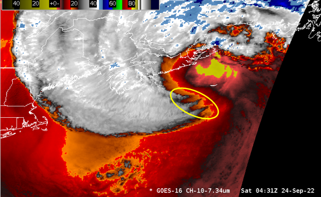
This is a sting jet at low-levels and is commonly observed with very strong winds at the surface.
Additional information on sting jets
Posted in: Cyclogenesis, GOES R, Heavy Rain and Flooding Issues, Hydrology, POES, Satellites, Tropical Cyclones, | Comments closed
ALPW analysis for the eastern Kentucky of 27-28 July, 2022
July 29th, 2022 by Dan Bikos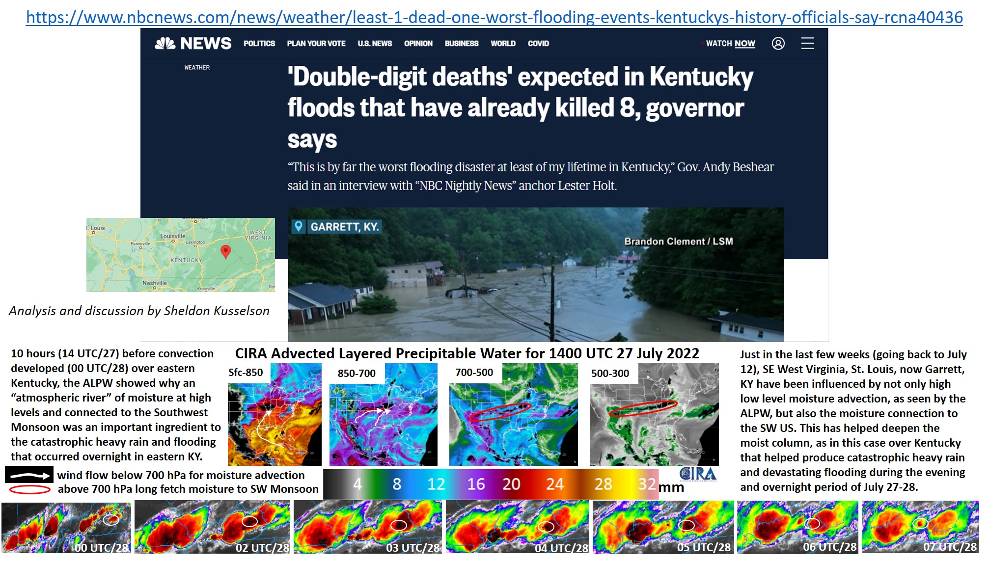
Posted in: Heavy Rain and Flooding Issues, POES, | Comments closed
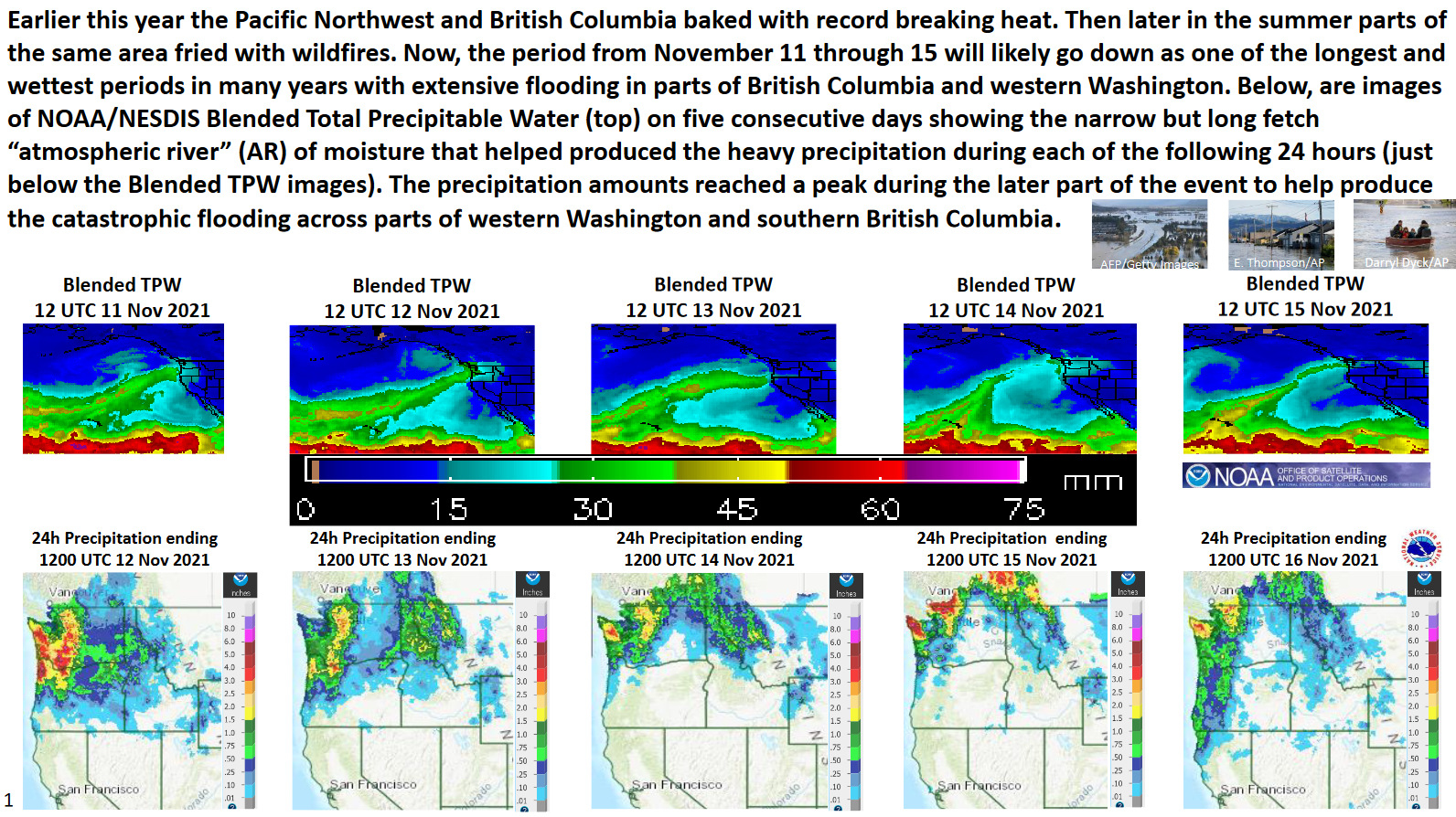
November 11-15, 2021 Atmospheric River event over the Pacific Northwest and British Columbia
November 22nd, 2021 by Dan BikosBy Sheldon Kusselson
Click on the image below:
Posted in: Heavy Rain and Flooding Issues, POES, | Comments closed