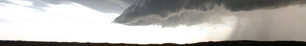
Elevated Mixed Layer event on 16 December 2019
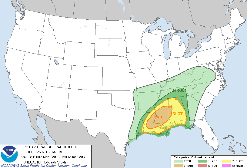
December 16th, 2019 by Dan BikosOn 16 December 2019, SPC issued an enhanced risk of severe thunderstorms for portions of Louisiana and Mississippi:
One of the favorable ingredients for this severe weather setup was the presence of an Elevated Mixed Layer (EML) which is depicted in the 12Z Jackson, MS sounding:
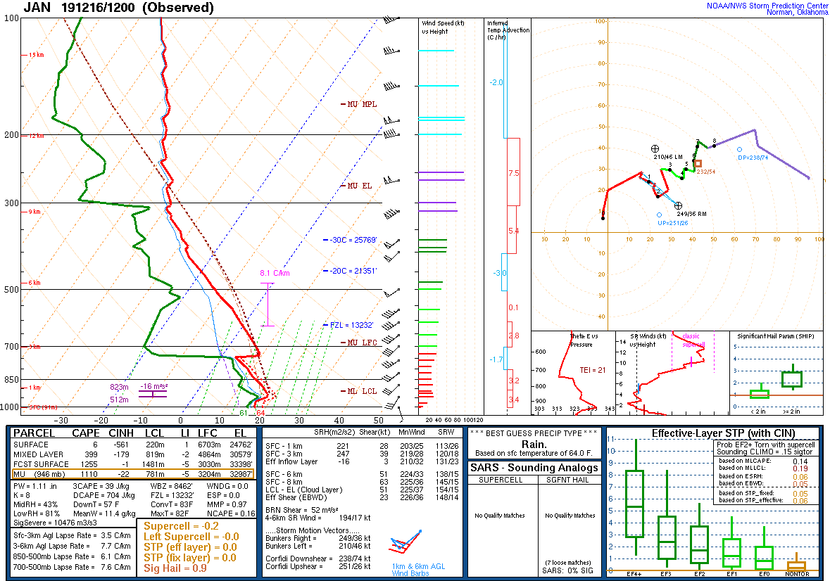
The EML is bounded between the capping inversion around 750 mb and the higher RH around 500 mb. Within this layer, the relative humidity is quite low with a source region off the elevated plateau of northern Mexico. Lapse-rates within this layer are relatively high, 700-500 mb lapse rate is 7.6 degrees C / km and the maximum is shown in the magenta layer on the sounding of 8.1 degrees C / km.
At times, the EML may show itself as a region of warmer brightness temperatures in the GOES 7.3 micron imagery. In this particular case, the region of warmer brightness temperatures may be traced back to diurnal heating from the previous day over the elevated Mexican plateau and advecting northeastward across Texas, Louisiana and Mississippi:
Clouds develop during the early morning hours which obscure the EML signature, however it may still be tracked via the Advected Layer Precipitable Water (ALPW) product:
ALPW is a product based on microwave instruments aboard polar satellites which can see through most clouds. The 700-500 mb layer is useful in that it depicts the source region of the dry air associated with the EML and it can be tracked towards Mississippi. This dry air exists underneath a moist air mass with origins from the Gulf of Mexico as seen in ALPW in the lower layers. ALPW allows a four dimensional perspective of assessing moisture in the vertical in time.
More information on EML tracking via satellite imagery and products:
Posted in: Convection, Severe Weather, | Comments closed
Australian Wildfires
November 18th, 2019 by Jorel TorresNighttime visible imagery (i.e. Near-Constant Contrast or NCC) clearly shows the Australian wildfires that are raging and ablaze in New South Wales, a state in southeastern Australia. NCC detects emitted lights from the fires, and at times shows the fire perimeter lines and reflected light from the extensive smoke plumes. The animation below displays nightly Suomi-National Polar-orbiting Partnership (SNPP) NCC imagery between 13-15Z from 11-13 November 2019. Cloud cover and emitted city lights from Sydney and Brisbane can also be seen. The moon phase and moon elevation angle are depicted in the bottom-left corner. The full moon phase of the lunar cycle and positive moon elevation angle imply the moon was above the horizon and provided adequate moonlight to illuminate atmospheric features (i.e. an ideal time to view NCC).
The smoke from the fires can be accentuated further utilizing an NCC enhancement technique. The AWIPS NCC color table scale can be customized to bring out certain atmospheric features in the imagery. In the images below, the default NCC 0-1 enhancement is compared to the NCC 0-0.5 enhancement on 12 November 2019. Notice how the NCC 0-0.5 enhancement brings out the smoke from the fires along with nearby cloud cover, but increases the saturation of city lights in comparison to the NCC 0-1 enhancement. For interested users, this quick guide provides steps on how to apply different enhancements to NCC imagery.
But how can one differentiate between emitted lights from fires to the emitted city lights? Users can overlay NCC with VIIRS infrared 3.74µm to identify fire hotspots at 375-m spatial resolution. NCC and VIIRS IR imagery are observed at ~1430Z, 13 November 2019 below. Hotspots (i.e. high brightness temperatures) and outlines of fire perimeters coincide with certain emitted lights. The emitted lights from cities disappear when compared to the thermal infrared.
To get an idea of the atmospheric instability near the fires users can display NUCAPS soundings; polar-orbiting satellite derived soundings that are optimal in clear-sky environments, and where in-situ observations are poor or limited. The NUCAPS sounding that is picked for this event is circled in blue (see below), observed right over one of the fires. It shows a moderately unstable, dry environment conducive for fire initiation and fire spread, where precipitable water values (derived from the sounding) are 0.31 inches. Note NUCAPS soundings are overlaid onto NCC imagery on 14 November 2019. NCC imagery observes smoke advection towards the coastline.


Downwind of the fire, another NUCAPS sounding is observed near the coastline (see blue circle). NUCAPS depicts a shallow inversion indicating a stable environment. Sounding is predominately dry, albeit there is slightly more moisture observed near the surface; increased precipitable water values (i.e. 0.55 inches) could be due to maritime influences and/or ‘fire produced water vapor advection’ towards the coastline.


Posted in: Miscellaneous, | Comments closed
Lake-effect snow from 7 November 2019
November 7th, 2019 by Dan BikosGOES-16 imagery depicts lake-effect snowbands over the western Great Lakes on 7 November 2019:
Upper left: 0.64 micron visible band
Upper right: 10.3 micron IR band with default color table (IR_Color_Clouds_Winter)
Lower left: 10.3 micron IR band with GOES Snow Squall color table
Lower right: Day Cloud Phase Distinction RGB
The 0.64 micron visible band provides detailed information on the location of the band, but reflectance values do not provide information about the intensity of the band.
IR imagery at 10.3 microns provides cloud top brightness temperatures, however lake-effect snowbands are typically shallow so that the difference in a precipitating lake-effect band and non-precipitating band is small. The small difference may not even be easy to identify if the color table has insufficient contrast around those brightness temperatures, as we see in the IR imagery with the IR_Color_Clouds_Winter color table. The IR imagery with the GOES Snow Squall color table helps somewhat but does not provide information on glaciation like the next product.
Finally, the Day Cloud Phase Distinction RGB provides the most useful information at a glance for assessing lake-effect snowbands. Not only does it identify the location of the snowbands, but also indicates clouds that are glaciated versus clouds that are not glaciated due to the 1.6 micron band. In this RGB product, glaciated clouds have transitioned from light blue to green (and perhaps even yellow if more developed although not shown in this case). This allows one to identify clouds that have glaciated and thus much more likely to be producing precipitation, even heavier precipitation if conditions are favorable.
The sounding from Alpena, MI provides useful information about the environment:
The sounding supports lake-effect snow in the region with the deeper PBL and large low-level lapse rates under the capping inversion. Note the winds are northwest in this layer, indicating this airmass was modified by sensible and latent heat fluxes from Lakes Superior and Michigan.
Posted in: Lake Effects, Winter Weather, | Comments closed
Water vapor imagery in an extremely dry airmass – 31 October 2019
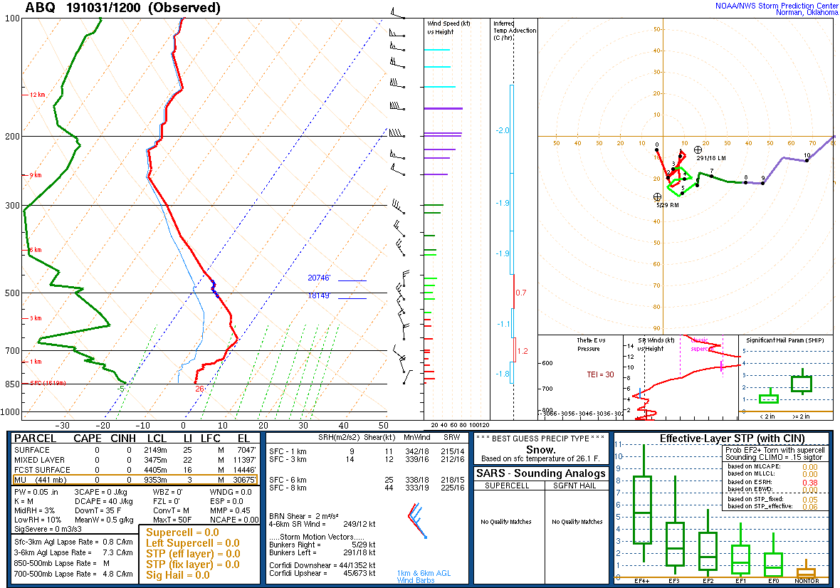
October 31st, 2019 by Dan BikosOn 31 October 2019 a very dry airmass existed over the southwest US. To illustrate the dry airmass, consider the sounding from Albuquerque, NM with a precipitable water amount of 0.05″ (1.27 mm):
The synoptic scale pattern was characterized by above normal PW in the east ahead of a trough, with below normal PW in the west behind the trough, as seen in the CIRA experimental TPW product:
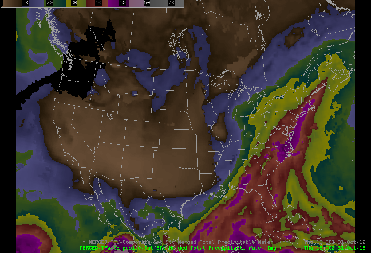
This experimental product combines retrievals from both polar orbiting and GOES satellites. Contrast this with the current operational blended TPW product on AWIPS which uses only polar orbiting satellite data.
Next let’s consider the GOES water vapor bands, normally the upper 2 water vapor bands (at 6.9 and 6.2 microns) do not see all the way to the surface due to water vapor absorption. Recall that on occasion the low-level water vapor band at 7.3 microns may see to the surface depending on how dry it is. In this extremely dry airmass over elevated terrain, what do the GOES water vapor bands show?
Upper left panel: GOES-16 Water vapor band at 7.3 microns
Upper-right: GOES-16 Water vapor band at 6.9 microns
Lower-left: GOES-16 Water vapor band at 6.2 microns
Lower-right: GOES-16 GeoColor
Note that we observe clear skies across this scene in the GeoColor product.
In the 7.3 micron (low-level) water vapor band, we readily observe the earth’s surface as it warms with daytime heating. You can compare the terrain features seen in this imagery with what is shown in GeoColor. The warmest brightness temperatures are observed due to a combination of locally highest elevations and a relative minimum in TPW. In the 6.9 micron imagery we observe brightness temperature maxima where we see mountain peaks across various ranges, particularly in New Mexico. Even at 6.2 microns we observe indications of diurnal heating and warmer brightness temperatures along various peaks in New Mexico.
To help explain why the imagery sees all the way to the earth’s surface we analyze the weighting function profile from the Albuquerque sounding (courtesy of CIMSS – https://cimss.ssec.wisc.edu/goes/wf/):
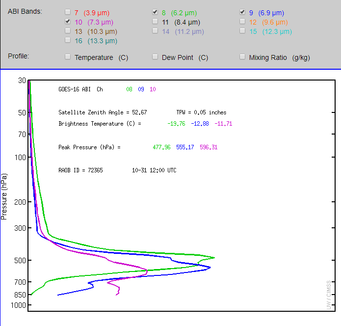
Typically the weighting function profile for water vapor bands on GOES does not extend all the way to the surface, however due to the extremely dry airmass in place, the 7.3 and 6.9 micron bands have contributions from the earth’s surface. In fact, the 6.2 micron band even had contributions at elevations just above Albuquerque which explains why higher mountain peaks, which would be above 850 mb, are being observed in the 6.2 micron imagery.
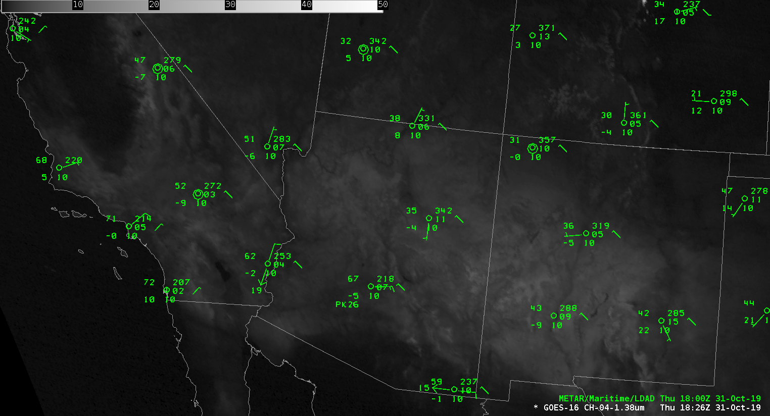
The 1.38 micron “cirrus” band also is significantly affected by water vapor absorption, which is why this band is typically used to highlight cirrus clouds since the earth’s surface is generally not seen due to significant water vapor absorption. In this particular case with an extremely dry airmass, the earth’s surface shows up readily across the region of interest:
Posted in: GOES R, POES, Satellites, | Comments closed
21 October 2019 – nighttime detection of fog and outflow boundaries
October 21st, 2019 by Dan BikosDuring the overnight hours of 21 October 2019, we analyze multiple applications of GOES imagery at night.
First, we look over the northeast where fog developed. Here is the GOES-16 nighttime microphysics product:
We observe large areas of fog (dull aqua) or low clouds (aqua) in Pennsylvania, New York, Vermont, New Hampshire and Massachusetts. Fog development in river valleys is particularly more easy to identify. Focus in over New York:
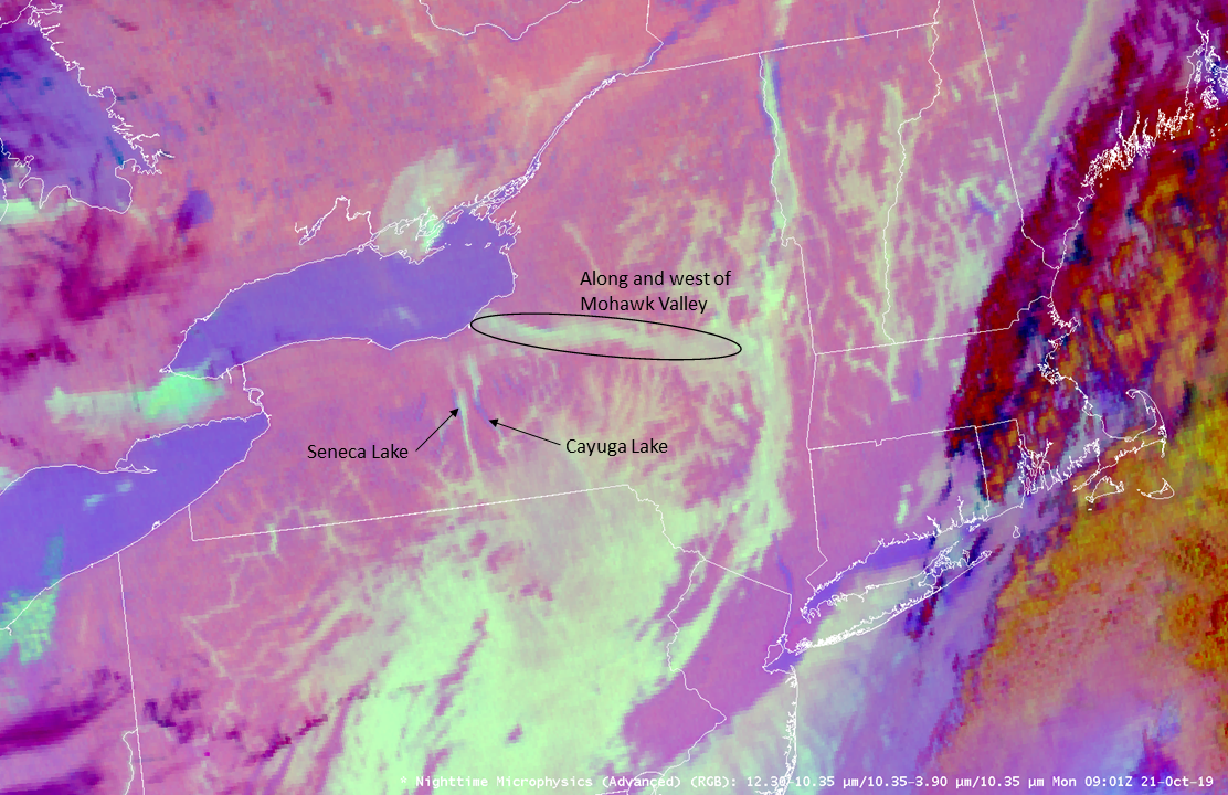
where the loop shows the westward movement of fog / low cloud from the Mohawk River Valley westward towards Lake Ontario. We also see the development of fog along Seneca Lake and Cayuga Lake.
Further southwest in Texas, severe thunderstorms developed during the evening hours of 20 October that continued through the overnight hours. The following GOES-16 imagery:
is a 4 panel display:
Upper-left: Split Window Difference / IR (10.3 micron) combination product
Upper-right: Nighttime microphysics RGB
Lower-left: IR (10.3 microns) with the default color table (IR_Color_Clouds_Winter)
Lower-right: Night Fog product (10.3 minus 3.9 micron)
Analyze the southern and western flanks of thunderstorms for regions of outflow (cooler brightness temperatures). Outflow boundaries can be important to analyze for mesoanalysis and potential future convection developing along or interacting with these boundaries.
Which of these imagery / products can you best identify the thunderstorm outflow air mass / boundaries with? Note that in some regions there are low clouds associated with the outflow. The IR imagery with the default color table has less contrast compared to other imagery / products for the detection of regions of outflow. Remember to look at other products for outflow detection at nighttime besides the IR (10.3 micron) band alone.
Posted in: Aviation Weather, Ceilings, Convection, Fog, Severe Weather, Visibility, | Comments closed