VISIT: Meteorological Interpretation Blog

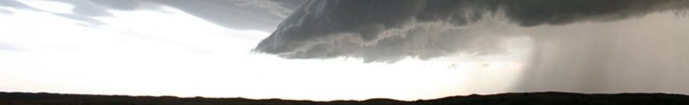
4 February 2019 significant ice storm in the Upper Great Lakes

On 4 February a shortwave tracked across the Upper Great Lakes towards the east, ahead of the shortwave, anomalously high moisture at low to mid-levels existed which contributed to a historic ice storm for the region.

The NWS forecast office in Marquette, MI has a great web-page summarizing this event including pictures and the meteorological environment:

This blog entry will focus on various satellite imagery and products, particularly those that highlight the anomalously high moisture for this event.

We lead off with a synoptic scale perspective of this event with the 3 Water Vapor bands from GOES-16 along with the Air Mass RGB:

The imagery clearly shows a shortwave in the North Dakota / Minnesota vicinity moving eastward. Ahead of this shortwave, precipitable water values were anomalously high, in fact record breaking TPW values were observed for this time of year in the Upper Great Lakes.  The anomalously high precipitable water values can be seen in the Advected Layer Precipitable Water product for the various layers.  Moisture plumes are observed with origins from the Gulf of Mexico in the SFC-850, 850-700 and 700-500 mb layers.  This shows that the moisture was relatively deep, particularly for this time of year in the Upper Great Lakes region.

An experimental product at CIRA that is still under development is the model minus ALPW PW for each layer.  For example, the HRRR minus ALPW PW for a given layer shows the difference between observations from ALPW versus different HRRR 3 hour forecasts (4 panel shows the same layer arrangement as the ALPW loop above). We primarily see positive values in the Upper Great Lakes region ahead of the shortwave, meaning that there’s more moisture in the HRRR 3 hour forecast compared to ALPW observations. A similar theme exists for the GFS (these are also 3 hour forecast fields).

Interestingly, the HRRR forecast a substantial ice storm, as seen in this set of forecasts:

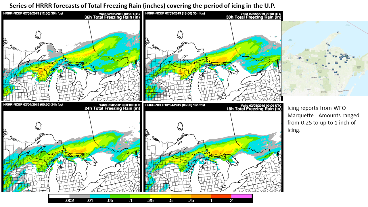
The anomalously high precipitable water played a key role in contributing to a historic ice event for this region, which typically observes snow during precipitation events this time of year.

The ALPW product is available in AWIPS from CIRA via LDM, however the model minus ALPW difference fields are not available since these are still in an experimental stage.

Posted in: Icing, | Comments closed

Observing sea surface temperatures from GOES and JPSS

Observing sea surface temperatures (SSTs) from satellite is an important aspect in weather forecasting for a variety of applications. Applications consist of (but not limited to) forecasting hurricane intensity, sea fog, and convection over the oceans. But remember, oceans are vast, making up ~70% of the Earth’s surface, and more importantly, oceans are remote, where surface observations are scarce. This is where satellite observations come into play, and can complement other data observations (e.g. radar, surface) to address certain weather forecasting applications.

Below, is a comparison between GOES16 SST and GCOM AMSR-2 SST observing the Gulf Stream on 6 February 2019. The comparison will highlight the benefits and limitations of each product.

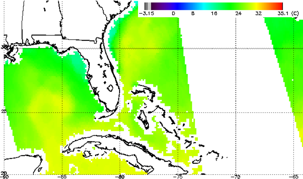
GOES16 – SST @1900Z, 6 February 2019

The geostationary product provides users hourly data (i.e. 15-minute data averaged into a 1-hour composite), at high spatial resolution of 2-kilometers. The product is derived from four, infrared, GOES16 ABI spectral channels: 8.4um, 10.3um, 11.2um, 12.3um. In the static GOES16 SST image below, notice the array of sea surface temperatures ranging from ~15°C to +30°C. However, also note the irregular, black colors, seen over the ocean. This irregularity is cloud cover and one of the limitations of GOES16 SST. Infrared satellite retrievals can only be produced in clear-sky environments.

GCOM AMSR2 – SST @ ~1843Z, 6 February 2019

Now in contrast to GOES16 SST, GCOM (a polar-orbiting satellite) AMSR2 SST is able to produce passive microwave SST retrievals in both clear-sky and cloudy environments. However, precipitating regions are problematic as well. In the imagery below, over the same domain, at approximately the same time (offset by 17 minutes), GCOM AMSR2 SSTs are observed. Notice there is also missing data (expressed in white colors over the ocean) in the imagery, however it is not due to clouds. The missing data is expressed via ‘data gap’, east of Florida. This is one of the limitations of polar-orbiters, in that polar-orbiters provide coverage up to ~2 times a day and GCOM AMSR2’s orbital swath does not overlap. Other limitations are GCOM AMSR2 SST’s coarser resolution (10 kilometers) and missing data over coastlines. Since microwave radiation is significantly different between land and ocean, SST retrievals that ‘do not’ have land in the field-of-view are considered.

GOES16 – SST Animation from 18Z, 6 February 2019 –> 16Z, 7 February 2019

For fun, here is an animation of the GOES SST, demonstrating its high temporal resolution, while observing the Gulf Stream moving near and around Florida: moving northward, up the southeastern coastline.

For interested readers, click on the following link to discover examples of polar-orbiting and geostationary data, combined together, to produce blended 5-km SST retrievals.

Posted in: GOES R, Miscellaneous, POES, | Comments closed

Arctic Blast in the Upper Midwest

A cold arctic air mass moved into the Upper Midwest the past two days (29-30 September 2019), providing extreme cold temperatures for several states, including North Dakota, Minnesota, Wisconsin, South Dakota, Iowa, and Illinois. Along with high winds, the calculated, respective, wind chills are even lower.

Satellite imagery, comprised of polar-orbiting and geostationary data, along with surface and upper air observations are used to demonstrate how cold it was for this portion of the United States. Images are provided between 29-30 January 2019.

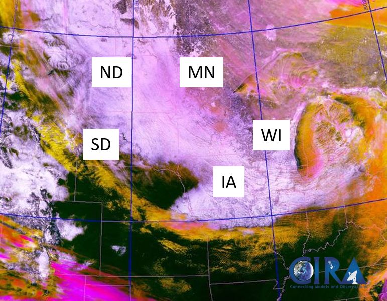
VIIRS Snow Cloud Discriminator: 1902Z, 29 January 2019

The VIIRS Snow Cloud Discriminator product (below) differentiates between snow cover (white), bare ground (dark green),  and low (yellow) – to – mid (orange) – to – high (pink) level clouds. Additionally, state abbreviations seen in the imagery are as follows: SD – South Dakota, ND – North Dakota, MN – Minnesota, WI – Wisconsin, and IA – Iowa. The static image shows the large areal extent of snow cover that resides in several states, as the arctic air mass advects over the domain.  In addition to the cold arctic air mass, snow cover played a role in the extreme, cold air temperatures observed in the Upper Midwest from 29-30 January 2019. To re-enlighten readers, snow cover traps longwave radiation (i.e. in the form of heat) that the Earth emits, and as a result, during the nighttime, near-surface air temperatures are predominately colder, since there is limited heat exchange between the surface and the atmosphere.

GOES-16 10.3um: 2147Z 29 January 2019 –> 1607Z 30 January 2019 

The animation below, shows infrared geostationary data, displaying cold brightness temperatures (ranging from -30C to -50C, light-to-dark blue and green colors) moving over the Upper Midwest. Notice how the cold air advection moves slowly southward, and appears slightly different in texture than cloud cover; cold air appears more smooth and uniform, than the rough, defined features of cloud cover. Additionally, cloud cover also develops and dissipates quickly over time, albeit, shows similar brightness temperatures to near-surface cold air. Note how the cold air extends all the way south to the Missouri/Iowa border, then stars to recede northward, when daytime solar heating begins (~13Z, 30 January 2019). The cold air extent also matches approximately to the snow cover extent observed by the VIIRS Snow Cloud Discriminator.

Surface Observations: 2158Z 29 January 2019 –> 1643Z 30 January 2019 

Furthermore, surface observations (provided from RAP Real-Time Weather) show the cold air advection from the event. Notice the strong northwesterly winds move through the domain, throughout time, and note the surface air temperatures (-40F or below, observed by some locations).

RAOB Soundings: KABR and KINL –> 12Z, 30 January 2019

To get an idea of how cold the air was not only at the surface, but aloft, one can refer to RAOB temperature and moisture soundings. Soundings below are both at 12Z, 30 January 2019, where the first sounding is from Aberdeen, SD (KABR), and the second is from International Falls, MN (KINL). Notice, how deep the arctic air mass is from Aberdeen, SD; the air mass extends from the surface – to ~550mb thick!

For interested readers, a Minneapolis, MN social media post of the event can be seen at the following link.

Posted in: GOES R, POES, Satellites, Winter Weather, | Comments closed

WS Harper Impacts on Northeast US

As Winter Storm Harper passed through the northeast United States, the storm brought heavy precipitation in the forms of snow, rain, and freezing rain that produced significant ice accumulation on the ground. Storm total snowfall, rainfall and ice accumulations were observed in Connecticut, Massachusetts, and Rhode Island. Specifically snow and ice accumulations ranged from 1-11 inches, and a trace-to-0.3 inches of ice respectively. Both accumulations on the roads, along with localized flooding from heavy rain can be hazardous to travelers. To access the storm observation reports, refer to the following NWS ‘Public Information Statement’ link.

The snow and ice accumulations were also observed from geostationary and polar-orbiting satellites, taken from before the storm (17 January 2019), and after the storm (21-22 January 2019).

Before the Storm: GOES-16, Band 5 – 1.6um @ 13-21Z, 17 January 2019

Geostationary imagery (i.e. animation) is at 1-kilometer spatial resolution, where the 1.6um spectral band is used. 1.6um, also known as the ‘Snow/Ice Band’, discriminates between the refraction components of water and ice. In the imagery, users would see liquid water clouds appearing bright, while ice clouds and ice accumulation on the ground (i.e. via snow or ice accumulation produced from freezing rain) will appear significantly darker. This is due to that ice absorbs radiation in 1.6um, where liquid water clouds reflect radiation at 1.6um. Also in 1.6um, land surfaces and bodies of water (i.e. lakes and ocean) exhibit great contrast as well. The animation below is before the storm, where it is used as a reference for readers. Notice no dark swaths of ice are observed in the states of Massachusetts, Connecticut and Rhode Island.

After the Storm: GOES-16, Band 5 – 1.6um @ 13-21Z, 21 January 2019

After the remnants of Winter Storm Harper passes through the New England area, notice an elongated, horizontal, dark swath observed in the imagery. Notice the dark swath earlier in the day, before mid-to-high level clouds obscure the surface features. Refer to the imagery inside the yellow ellipse.

After the Storm: GOES-16, Band 5 – 1.6um @ 13-21Z, 22 January 2019

The very next day is also explored, since the day predominately encapsulates a cloud-free atmosphere, before high-level cirrus clouds move over the domain. The dark swath can be seen throughout portions of Connecticut, Massachusetts and Rhode Island.

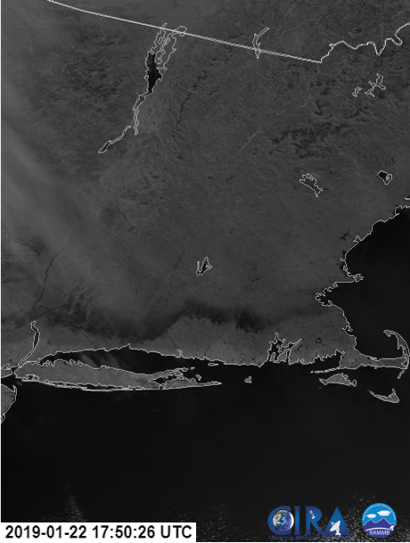
After the Storm: NOAA-20, I-3 Band – 1.6um @ 1750Z, 22 January 2019

Need a better spatial resolution of the dark swath? Refer to polar-orbiting satellite imagery. NOAA-20 VIIRS imagery data is produced at 375-meter spatial resolution, and provides more detailed surface features, although the temporal resolution of polar-orbiters are infrequent.

Social media highlighting the ice accumulation can be seen via the following links: photo, and video.

Posted in: GOES, Icing, POES, Winter Weather, | Comments closed

Winter Storm Harper

A large low pressure system, slammed into the western United States (US), bringing heavy rain and snow, high winds, along with producing blizzards (for the Sierra Nevadas) and localized flooding for low-lying areas.

The areal extent of the system is seen via ‘Preliminary, Non-Operational‘ GOES-17 Day Cloud Phase Distinction RGB (below) at 1925 UTC, 16 January 2019, as the storm approached the Western US.  The RGB differentiates between liquid water clouds (blue), glaciated clouds (green) and mid-to-high level ice clouds (yellow-to-red clouds). Note the elongated rope cloud, associated with the cold front, in the southwest portion of the image, depicted in quasi-linear blue and green colors.

The winter storm can also be seen via Advected Layered Precipitable Water (ALPW) product, that is derived from polar-orbiting satellites and identifies areas of high moisture content and moisture transport that can lead to heavy precipitation and flooding. Animation below, shows the ALPW product from 06 UTC, 16 January 2019 –> 15 UTC 17 January 2019, highlighting Winter Storm Harper as it moves into California, Oregon and Washington. The colorbar is at the top of the animation depicting 0-32 mm (black to pink colors) precipitable water values. ALPW is different from Total Precipitable Water (TPW) products, in that ALPW identifies precipitable water from four atmospheric layers (surface-850mb, 850-700mb, 700-500mb, and 500-300mb), rather than specifying the total precipitable water values for the entire atmospheric column.

In this case, as Winter Storm Harper approaches land, notice high concentrations of precipitable water between the surface-to-500mb (blue/aqua colors), and significantly lower precipitable water concentrations in the upper atmosphere (i.e. 500-300mb, grey to black colors). Also note an elongated atmospheric river on the southeast side of the low pressure system. The atmospheric river moved into and impacted south-central and southern California, where the Sierra Nevadas experienced heavy snowfall rates (up to ~3 inches per hour) and high snow accumulations.

Speaking of the Sierras, earlier this morning there were reports of thundersnow in the Sierras. Reports were near Mammoth Mountain, CA, in which the ‘Preliminary, Non-Operational‘  GOES-17, Geostationary Lightning Mapper (GLM) detected lightning signatures near Mammoth Mountain. Animation below shows GOES-17 GeoColor imagery overlaid by GLM – Group Flash Count Density signatures. Time period observed is between 12-1445 UTC, 17 January 2019. Notice the lightning signatures observed in the Sierras that experienced thundersnow.

Winter Storm Harper plans to create more havoc throughout today and into the weekend, moving into and impacting the Rocky Mountains, Central Plains and Eastern United States.

Posted in: GOES R, Heavy Rain and Flooding Issues, Hydrology, POES, Satellites, | Comments closed