VISIT: Meteorological Interpretation Blog

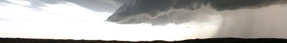
Dragon Bravo Fire, Arizona

At the time of this blog entry, the Dragon Bravo Fire burned 130,000 plus acres along the Grand Canyon National Park’s North Rim and is only ~13% contained. The fire initiated on 4 July 2025 and several structures along the North Rim, including the historic Grand Canyon Lodge, have already been destroyed. The cause of the fire was due to lightning. Prolonged hot, dry and windy conditions aided in the fire spread.

The high temporal resolution GOES ABI captured the rapid fire spread throughout the course of a week and half, from 24 July – 4 August 2025. Notice the active hotspots (i.e., white and red pixels) and the increased fire spread to the north.

GOES-18 ABI 3.9 um hourly observations from 0000Z, 24 July 2025 to 0000Z, 4 August 2025

VIIRS 3.7 um (I4) imagery zooms in on the finer details of the hotspots and the advancing fire perimeter during a similar time period. VIIRS observes these features at a high spatial resolution of 375-m compared to the coarser GOES 2-km resolution. The shortwave infrared imagery from VIIRS and GOES can be used in complement with one another during the day and night to observe fire hotspots, along with other thermal anomalies.

VIIRS 3.7 um (I4) observations from ~9Z, 24 July 2025 to ~9Z, 3 August 2025

Another way to view the Dragon Bravo Fire is from the VIIRS Day Fire RGB that utilizes three individual spectral bands (I4 – 3.7 um, I2 – 0.86 um, and I1 – 0.64 um) to detect fires, monitor vegetation changes and observe smoke. The RGB has the same 375-m spatial resolution and captures the active fires, burn scars and smoke produced from the Dragon Bravo Fire. Note, one of the limitations of the RGB is that the dataset can only be used during the daytime and is not available at night.

VIIRS Day Fire RGB observations from ~20Z, 24 July 2025, to 21Z, 3 August 2025

Posted in: Uncategorized, | Comments closed

A Tropical Upper Tropospheric Trough (TUTT) in Florida

The Tropical Upper Tropospheric Trough – TUTT (Sadler, 1976) is a trough or cyclonic circulation in the mid-upper troposphere located in tropical locations. Sadler defined the TUTT as an upper trough that lies between upper ridges in the subtropics and ridges in tropical locations. The TUTT is a complex system that often enhances convection along its periphery and limits it near its center. However, strong TUTTs can also enhance convection near their centers, given destabilization stimulated by the cold air present in their cores. In rare occasions, a strong TUTT that develops weak upper winds and strong convection near its center can yield to a cyclonic circulation at the surface that eventually triggers tropical cyclogenesis.

GOES-19 6.9um channel satellite imagery (link to quick guide) shows a TUTT located over the Bahamas and southeast Florida on the morning of 23 July 2025. The satellite presentation of the system shows a classical TUTT, characterized by strong convection along its periphery and a minima in convection near its cyclonic core. Animating water vapor channels such as the 6.9um one is an effective method to observe systems located in the mid-and upper troposphere, as these channels capture the motion of water vapor in these layers. The following animation shows the cyclonic rotation associated with the TUTT, which centers near Andros Island in the northwest Bahamas. It also shows convective tops in the periphery of the TUTT in shades of light gray and blue (brightness temperatures near and below -30°C), which rotate cyclonically around the center. The orange coloration (warmer temperatures) indicates drier air, which was entering the system from the northeast. When dry air in the mid troposphere is present very close to convection, it can enhance its strength by stimulating evaporation. This yields to cooling and, in turn, enhances vertical motion in the storms. The common presence of dry air near the center of a TUTT is one reason why they are often associated with strong convection that contains lightning, large rainfall rates and sometimes gusty winds.

The TUTT can also be seen on other satellite products. The following animation shows CIRA’s GeoColor product. In order to evaluate the location of thunderstorms, CIRA’s GLM Optical Energy product (link to quick guide) has been overlaid. The GeoColor is able to measure the surface and low-level clouds when higher clouds are not obscuring the view. This capability illustrates that the cyclonic rotation evident in the 6.9um channel is not occurring at the surface. In fact, the movement of low-level clouds is different. Lightning data from the GLM also confirms the presence of thunderstorms. The stronger storms are occurring over and off the coast of southeast Florida, in the periphery of the TUTT, given the interaction of three processes that are interacting to highlight ascending motions: (1) horizontal moisture gradients in the mid troposphere, (2) upper jet dynamics and (3) TUTT propagation. Role of moisture gradients: In the northwest portion of the TUTT, the dry air intrusion from the northeast of the TUTT (described in the previous paragraph) meets the very moist air mass located near southeast Florida, highlighting evaporative cooling processes and vertical motions. Role of upper jet dynamics: stronger upper winds over Florida, evidenced by the fast motion of the higher clouds, produces horizontal wind gradients that highlight ascent. Role of TUTT propagation: rapidly decreasing geopotentials in the mid-troposphere, as the TUTT approaches Florida from the southeast, enhance ascent. A fourth factor (not shown in these animations) is the presence of high values of available moisture over Florida. For this, precipitable water products are recommended. The combination of all of these processes yields to strong thunderstorms with frequent and dense lightning.

Not related to the TUTT but also of interest, CIRA’s GeoColor product shows that a Saharan Air Layer Intrusion is propagating northwestward in eastern portions of the domain. How can we tell? By the presence of a milky or whitish color shade in eastern portions of the image, which contrasts with the dark blue color of the ocean elsewhere in the figure. This contrast is more defined near sunrise. The reason is that the radiation beams returning to the satellite from the earth-ocean-atmosphere system have to travel in a low angle to reach the satellite. This forces them to encounter larger amounts of dust before reaching the satellite. The scattering of solar radiation caused by the dust produces the bright coloration that appears in CIRA’s GeoColor product.

An additional impact of the TUTT is the modulation of vertical wind shear, due to the vertical differences in wind directions and speeds in different quadrants of the TUTT. This has an impact in convection. The Day Cloud Phase Distinction RGB (link to quick guide) product is very useful to understand cloud types, and animating it shows how clouds at different levels move. It can provide a qualitative assessment of wind shear. It also illustrates convection types. Shallow convection in the tropics consists of water clouds, which appear blue and green. Yellows and oranges show ice clouds, which relate to deep convection and cirrus. The following animation shows this product from 12:50 through 18:00 UTC, capturing the diurnal cycle of solar heating. The impacts of the TUTT and how it relates to the diurnal cycle and to the Saharan Air Layer are described in the animation.

Reference:

James C. Sadler, “A Role of the Tropical Upper Tropospheric Trough in Early Season Typhoon Development,” Monthly Weather Review, October 1976, Volume 104, pp. 1266–1278.

Posted in: Uncategorized, | Comments closed

Alaska Heatwave

During mid-June 2025, National Weather Service (NWS) Fairbanks, AK, issued Heat Advisories for the first time over the Alaskan Interior, where above normal temperatures were expected over the region. The newly implemented advisory system for Alaska was a way to help better communicate heat impacts to the general public. An example of a heat advisory issued by NWS Fairbanks, AK, via social media, can be found below.

The prolonged summer heat lead to significant snowmelt and the reduction of existing snow cover over northern Alaska, that included the Brooks Mountain Range. JPSS polar-orbiting satellites observed the snowmelt over the course of two weeks, captured by the VIIRS GeoColor product at 750-m spatial resolution. The daytime animation below shows the reduction of the snow areal extent, while observing fires and smoke, in addition to multiple rounds of convection during the time period. Note, the daytime images were taken each day, between ~19-02Z. Refer to the blue rectangle within the animation.

VIIRS GeoColor observations over northern Alaska from 9-24 June 2025

Another way to view the rapid melting of snow is from the VIIRS Snowmelt RGB at 750-m spatial resolution. The RGB utilizes the VIIRS 1.24 um channel that is not available on GOES satellites, and is highly sensitive to snow properties, such as grain size and relative wetness. In a qualitative way, the VIIRS Snowmelt RGB observes wet/old snow (dark blue colors) over northern Alaska that could lead to increased snowmelt runoff and flood potential. Dry/new snow appears brighter (cyan colors) in the imagery; as the snow ages over time, the imagery reflectance will gradually decrease. Additionally, the RGB differentiates between liquid clouds (white), thick ice clouds (shades of cyan), thin ice clouds (bluish-white) and vegetation (brown/green colors). The VIIRS Snowmelt RGB image comparison below highlights the existing snow cover on 9 June 2025 and the remnant snow cover seen on 17 June 2025.

Comparison of the VIIRS Snowmelt RGB on 9 June and 17 June 2025

Posted in: Uncategorized, | Comments closed

Galvez-Davison Index (GDI) as another tool to forecast convection in North America

June 13th, 2025 by José Manuel Gálvez

The Gálvez-Davison Index (GDI) (Gálvez and Davison, 2016) was developed by José Gálvez and Mike Davison at NOAA’s Weather Prediction Center in 2014, to improve the detection of environments favorable for tropical convection [Online access: https://www.wpc.ncep.noaa.gov/international/gdi/ ].  However, its skill does not only limit to tropical locations. It extends into mid-latitudes during the warm season. This means that it can be used in the United States during the summer, particularly in regions where warm and moist air masses develop.  This short blog uses satellite imagery to show a simple example of (1) how the GDI has skill in parts the United States during the warm season and can be used as a forecasting tool and (2) the importance of incorporating an analysis of atmospheric dynamics to better assess where convection might form or continue.

Like most stability indices, the GDI is not a standalone index and should be analyzed in combination with atmospheric dynamics.  The GDI only describes the static environment where convection might form, given that its calculation does not consider wind information.  Consequently, it only provides information about whether or not atmosphere is capable of hosting convection and rainfall, but it does not really tell the forecaster whether there convection triggering mechanisms will be present. This is where an analysis of flow dynamics will enhance convection forecasts.

Let’s start with a quick description of the Galvez-Davison Index (Figure 1).  The GDI is computed using temperatures and mixing ratios from 4 atmospheric levels: 950, 850, 700 and 500 hPa.  It represents three processes that are summarized in three sub indices:  (1) The CBI describes the availability of heat and moisture in the 950-500 hPa column, (2) the MWI incorporates the impacts of stabilization by warm air masses in the mid-troposphere and (3) the II represents the drying and stabilizing impacts of thermal inversions in the lower and low to mid troposphere.

How to interpret GDI values? A general interpretation diagram is available in Figure 2. The GDI is dimensionless.  Low values relate to shallow convection and very little precipitation, while higher values suggest a higher potential for deep convection. In the color scale we often use, the chances for deep convection generally increase when greens and yellows appear (GDI=15 to 35), and once oranges and reds appear (GDI>35), the potential for deep convection increases. A potential for heavy rain producing convection appears as well when GDI approaches 35, and increases with higher values.

For a quick look into the skill of the GDI in North America, a random day when GDI was high in the United States and convection was present was chosen: 12 June 2025.  Figure 3 summarizes the GDI field circa 18 UTC. This is close to midday or the early afternoon in the United States.  We are using GDI calculated with GFS model data, 18 hour forecast, using the software Wingridds.  According to the figure, deep convection is likely to develop in points A, B and D; and to a minor degree in point C.  A higher chance for deep convection appears in region E, in south-central Mexico, where GDI values are high.

Now let’s look at where the convection was actually forming around 18 UTC using satellite products.  We will use an animation of the 10.3 um channel or one of the longwave IR channels available in GOES-19 presented in Figure 4.

Figure 4. Animation showing the 10.3 um long wave IR band of GOES-19. Source: CIRA Slider.

Thanks to the satellite loop, we can verify that the GDI seems to be capturing the development of deep convection in points A and D. Using this band and the chosen color palette, we can generally interpret the presence of deep convection by oval-shaped areas colored green, yellow, orange and red that are generally growing. These colors represent cold cloud tops, which are present in deep convective cells. The strongest system appears to be located in southeast Texas in point A, while in point D, the satellite signature suggests diurnal convection already developing in Florida. But what is happening in the other points? And what about the deep convection forming in the Rocky mountains, west of point C, while nothing is occurring at point C itself where the GDI is higher? Let’s start answering this by a quick analysis of atmospheric dynamics.

Figure 5 is very similar to Figure 3, but contains additional model information to interpret atmospheric dynamics.

Incorporating an analysis of the structure of the upper flow (yellow streamlines and wind barbs) as well as the low-level flow (black streamlines and barbs) provides an important amount of additional information. It shows that the convection in point A is also being stimulated by a robust upper trough extending from eastern Nebraska across southwest Oklahoma into south-central Texas. Embedded in this large upper trough, a negatively tilted short wave trough structure (light blue dashed line) is propagating northeastwards across east Texas. The term “negatively tilted” trough is generally used to describe a trough that has its warm tier ahead or downstream of its cold tier. This configuration tends to associate with enhanced upper divergence (white contours) and enhances ascent in the column. In the low-levels, the upper trough has induced a surface trough and it associates with enhanced moisture convergence (red contour). Thus according to the model, there is important dynamical forcing in point A. Satellite imagery in Figure 4 supports this, although precise location of the strongest convection does not match what the model suggests with high precision. This partly relates to complex mesoscale structures associated with the mesoscale convective system in southeast Texas. But what is happening in the other points? Let’s dive into the Day Cloud Phase Distinction RGB (Figure 6) to explore convective initiation.

Figure 6. Animation showing the Day Cloud Phase Distinction RGB (JMA color table) available from GOES-19 data. It also contains CIRA’s GLM Group Energy Density product overlaid, to detect thunderstorms. Source: CIRA Slider.

The Day Cloud Phase Distinction RGB is a great tool to detect convective initiation, or the beginning stages of clouds growing vertically into mid and upper portions of the troposphere. Clouds that contain water droplets look cyan in this product. But when convection initiates and clouds grow, they reach higher altitudes where temperatures are colder. As a result, they develop ice. In this RGB, thick ice clouds appear yellow. The animation shows that in points B, E and F, convection is only starting to form. This suggests that the diurnal cycle in these locations could matter. In point C, however, atmospheric dynamics seem to be tampering the impacts of high GDI values. Looking back into the flow analysis presented in Figure 5, region C (eastern Colorado and west Kansas) lies under an upper ridge and in a region where low-level moisture convergence is not enhanced. Low-level divergence could be even present, but it is not plotted. To the west of point C, however, deep convection is rapidly forming along the Rocky Mountains. Figure 5 suggests that this could be responding to enhanced low-level convergence (red contours) and an approaching short wave upper trough marked with a yellow dashed line.

Since we would like to evaluate the role of the diurnal cycle, lets look at the evolution of convection later in the day using a similar product, but covering the 19-23 UTC period (Figure 7).

Figure 7. Similar to Figure 6, but covering the 19-23 UTC period. Source: CIRA Slider.

Once we look at the evolution past 19 UTC, we verify that – indeed – the diurnal cycle of solar heating seems to play a role as a convection trigger. Rising thermals enhanced by solar heating past 19 UTC have the ability to break the cap or convective inhibition region in the lower troposphere, reaching altitudes where they acquire the ability to use high GDI to produce convection. This is especially true in mountainous regions such as Mexico and the Rocky mountains (points G and H), given the enhanced role of diurnal heating in elevated terrain and continental regions. The western location of these mountain ranges also plays a role in the later occurrence of convective initiation. But evaluating the dynamics also matters. In points G and H, added only in Figure 7, enhanced low-level moisture convergence associated with moist diurnal upslope breezes seems to be important. In point B, convection developed in a scattered to isolated manner. Looking at the GDI alone could had been a little misleading. But when considering atmospheric dynamics, the basic analysis that Figure 5 allows suggests that there might be a general lack of significant dynamical forcing. Yet, the confluence of low-level flow in eastern Tennessee apparently resulted in a region of enhanced low-level moisture convergence producing the cluster of scattered thunderstorms in the region.

Note on the Day Cloud Phase Distinction (JMA) Product: A final aspect of the Day Cloud Phase Distinction Product, not related to the GDI, is the change of coloration as the sun sets. The reason is that this product uses reflective bands that depend on solar radiation. However, areas with cold cloud tops are visible throughout the night, but acquire a red coloration. This is caused by the 10.3 um band being included in the red component of the RGB. During nighttime, the green and blue components of the RGB disappear due to the lack of solar radiation. Only cold cloud tops are visible at night, and they look red.

Figure 8. Recipe to code the Day Cloud Phase Distinction RGB. Source: CIRA.

Thank you for reading.

Posted in: Uncategorized, | Comments closed

11-15 May, 2025 Flooding Event in the Mid-Atlantic and Southeast USA

by Sheldon Kusselson

Posted in: GOES, Heavy Rain and Flooding Issues, Hydrology, POES, Satellites, Uncategorized, | Comments closed