VISIT: Meteorological Interpretation Blog

NOAA-21 Designated as the Primary Satellite of the JPSS Constellation

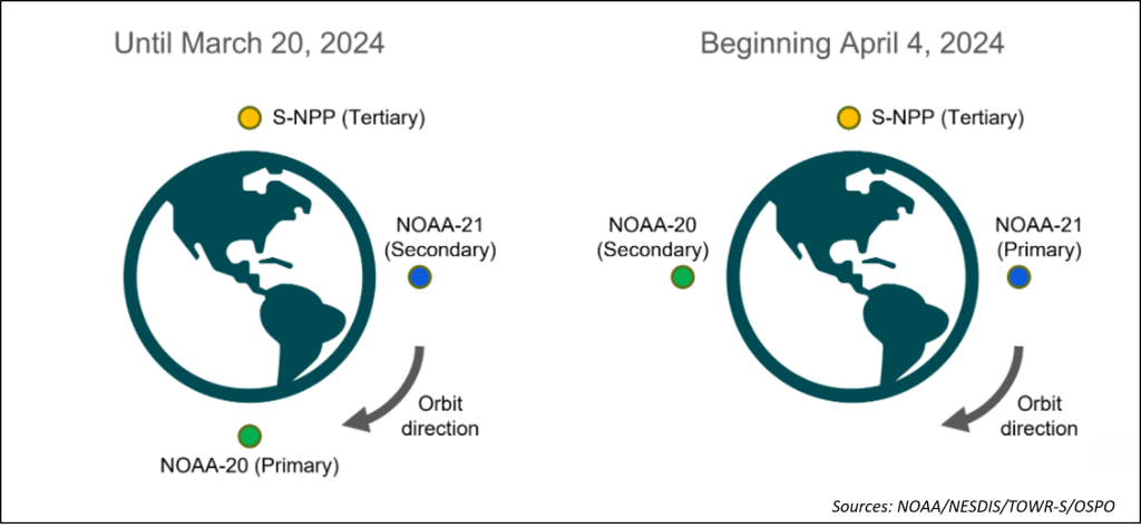
During March 2024, NOAA-21 was declared the primary satellite of the Joint Polar Satellite System (JPSS). In early April 2024, NOAA-20 (newly designated as the secondary satellite) completed its orbital shift placing NOAA-20 a half-orbit (~50 minutes) a part from NOAA-21. The tertiary satellite, SNPP, is now positioned a quarter-orbit between NOAA-21 and NOAA-20. A schematic below displays and compares the old JPSS orbital configuration (pre – 20 March 2024) to the finalized orbital configuration (4 April 2024).

For users, how does the new orbital configuration appear in the imagery? A CONUS perspective of VIIRS 11.45 µm swaths from NOAA-21, SNPP and NOAA-20 are seen on 10 April 2024. Notice the JPSS orbital sequence (observed from east coast to west coast) starts with NOAA-21, then ~25 minutes later SNPP, then NOAA-20 ~25 minutes after that. Afterwards, a 50 minute data gap occurs, then the sequence repeats.

The same orbital sequence can also be seen over Alaska. Refer to the 2 May 2024 VIIRS Snow/Cloud Layers animation that shows the sea ice coverage over the Bering and Chukchi Seas and low/high clouds and snow over the Last Frontier State.

Posted in: Miscellaneous, POES, Satellites, VIIRS, | Comments closed

Flooding in the UAE and Oman

During mid-April 2024, unprecedented flooding occurred in the Middle East, specifically in the countries of the United Arab Emirates (UAE) and Oman. Over the course of a few days, a series of storms produced significant precipitation totals that pummeled the region, which led to extensive flooding that shut down schools, grounded or diverted flights, and caused fatalities.

The Meteosat-9 SEVIRI 6.25 µm captured numerous storms that passed through the region from 14-16 April 2024. The upper-level water vapor channel also observed a strengthening low-pressure system that enhanced precipitation in the UAE and Oman during 15-16 April 2024. In the water vapor animation below, notice that several storms develop on the southeast side of the upper-level trough.

With an emphasis on 16 April 2024, a SEVIRI Day Cloud Phase Distinction RGB animation can be seen, that captures storms that develop and spread across eastern Saudi Arabia, Qatar, the UAE and Oman. At ~12Z, a north-to-south line of convective initiation develops in the UAE/Saudi Arabia region, and advects eastward towards Oman. Outflow boundaries (seen in cyan) are also seen moving southward in eastern Saudi Arabia.

JPSS polar orbiting satellites observed the severe weather as well. Although, the polar-orbiters have a coarse temporal resolution (compared to the geostationary satellites), they provide high spatial resolution imagery at 375-m. NOAA-20 and NOAA-21 VIIRS Day Cloud Phase Distinction RGB imagery observed the storms at 0930Z and 1019Z, 16 April 2024.

During the same time period, the SEVIRI Dust RGB observed areas of blowing dust (i.e., in bright magenta/pink) in southern Saudi Arabia. Dust associated with the outflow boundaries can also be seen (pink/purple shades).

The Blended Total Precipitable Water (TPW) product provided insight of the moisture content within the region. Blended TPW observed high precipitable water values (2+ inches seen in red colors) in the southeastern part of the Arabian Peninsula. The rich moisture plumes aided in the development of heavy precipitation that led to flooding in the region. Note, Blended TPW observes the total precipitable water throughout a column in the atmosphere and does not identify where the moisture is located aloft (e.g., 850mb-700mb layer).

Using the NOAA Satellite Proving Ground Global Flood Products Archive, one can get a sense of the flooding that transpired in the UAE.  A ‘Before’ (7 April 2024) and ‘After’ (17 April 2024) VIIRS Flood Map image comparison shows the extent of flooded pixels (yellow to red pixels) near and southwest of Abu Dhabi, UAE. Noticeable new areas of inundation from the heavy precipitation event can be seen inland, and along highways in the 17 April 2024 – VIIRS Flood Map image. The VIIRS Flood Map product has a 375-m spatial resolution.

Posted in: Convection, Dust, GOES, Heavy Rain and Flooding Issues, Hydrology, POES, Satellites, Severe Weather, VIIRS, | Comments closed

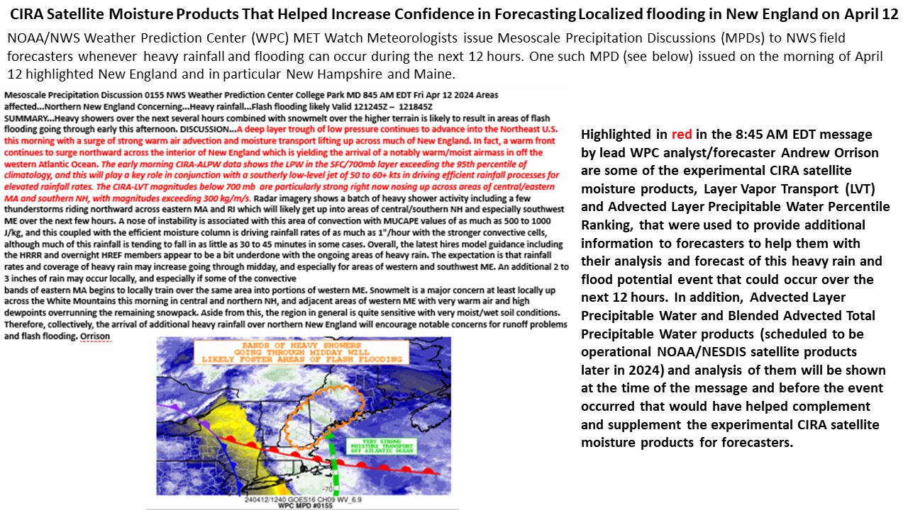
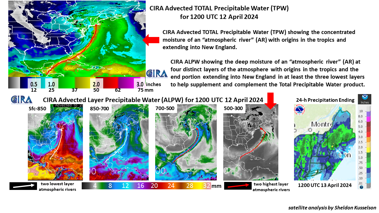
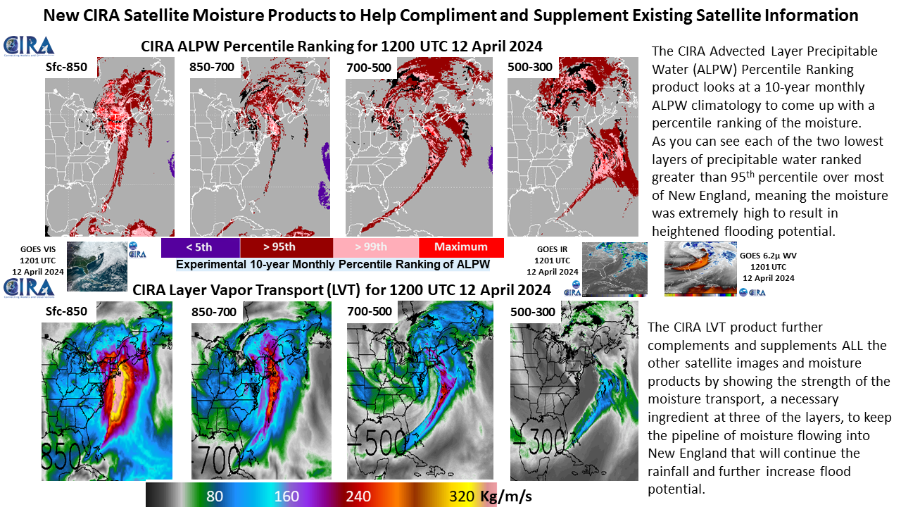
CIRA Satellite Moisture Products – New England localized flooding on April 11-12, 2024

By Sheldon Kusselson

Animations:

ALPW

Layer Vapor Transport

Percentile Ranking

Posted in: Heavy Rain and Flooding Issues, Hydrology, POES, Satellites, | Comments closed

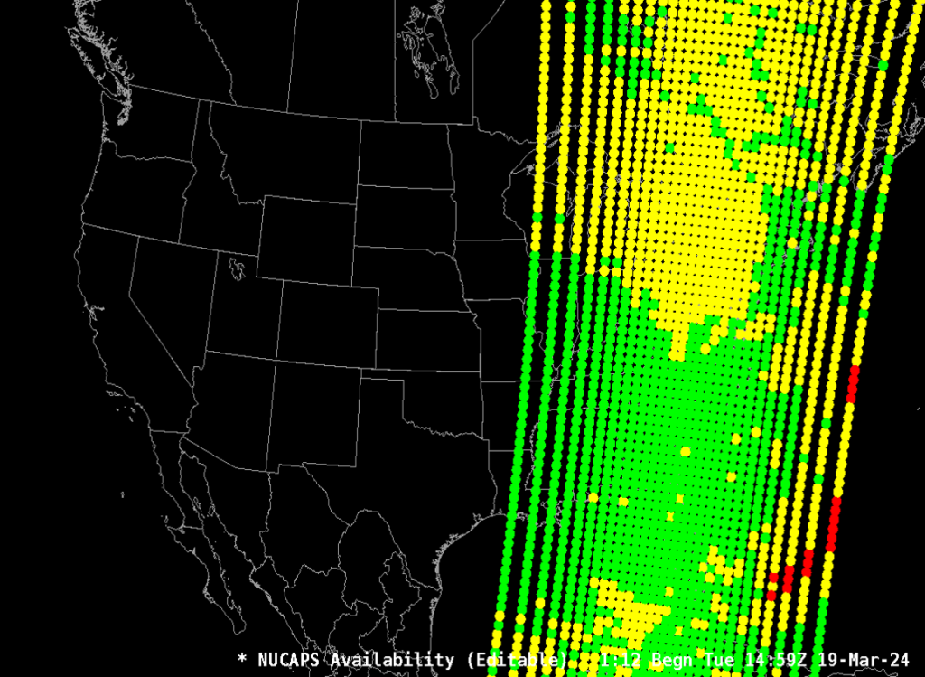
Metop-C NUCAPS Soundings Available in AWIPS

In complement to the NOAA-20 NUCAPS soundings, National Weather Service (NWS) forecasters now have access to another set of satellite-derived soundings from the European Metop-C satellite in AWIPS-II. As of 11 March 2024, the Metop-C NUCAPS soundings are accessible via Satellite Broadcast Network (SBN) across the CONUS (and globally). The Metop-C soundings provide mid-morning overpasses over the Lower-48 (i.e., ~14Z-17Z, from east coast to west coast) to assist in analyzing the pre-convective environment and provide overpasses during the late evening/overnight hours (i.e., ~01Z-05Z, from east coast to west coast). A swath of Metop-C NUCAPS profile sounding points can be seen below.

Metop-C NUCAPS soundings over the eastern U.S. at ~15Z, 19 March 2024. 

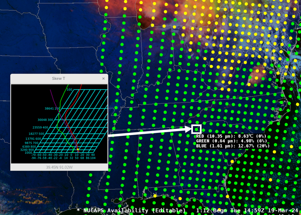
Over the same time period, GOES-16 Day Cloud Phase Distinction RGB imagery was overlaid onto the Metop-C NUCAPS soundings, and show a clear-sky environment for a good portion of the southeast U.S. Employing the Pop-Up Skew-T function in AWIPS-II, a green sounding point (i.e., an indication of a successful infrared and microwave NUCAPS retrieval) was selected near the South Carolina and Georgia border, that observes a dry boundary layer near the surface and aloft.

A Metop-C NUCAPS profile displayed near the Georgia and South Carolina border at ~15Z, 19 March 2024.

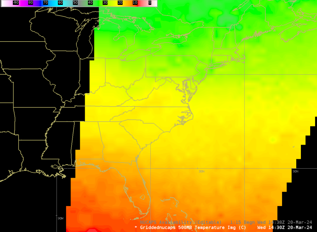
Gridded NUCAPS (i.e., plan-view displays of the temperature and moisture fields) from Metop-C are also available for user consumption. An example of Gridded NUCAPS over the east coast can be viewed below.

Metop-C Gridded NUCAPS 500 millibar (mb) temperatures at ~1439Z, 20 March 2024.

At the time of this blog entry, there is not a way to differentiate between NOAA-20 and Metop-C NUCAPS soundings in AWIPS-II. In the meantime, forecasters can identify and differentiate the orbit tracks by referring to the NOAA VLab Polar Planner Tool and the SSEC Polar Orbit Tracks website.

In the incoming months, forecasters can also look forward to another set of satellite-derived soundings from NOAA-21 to become available in AWIPS-II.

Note, users can access NUCAPS soundings online via NOAA OSPO Global Map and the Gridded NUCAPS datasets over CONUS via RealEarth and NASA SPoRT webpages.

Posted in: AWIPS, Data Access, News of Interest, POES, Satellites, | Comments closed

Texas Fires

Fires erupted over the Texas Panhandle during the last week of February 2024. The fires burned over 1+ million acres, where the Smokehouse Creek Fire became the largest fire in Texas state history. Videos of the fires and drone footage of the destruction were vast. Geostationary and polar-orbiting satellites captured the event over the course of the week.

The GOES-16 Fire Temperature RGB observed the rapid fire spread from 1756Z – 2056Z, 27 February 2024.  Refer to the animation below.

During the same timeframe, the NOAA-20 and SNPP VIIRS Fire Temperature RGB captured the fires at 1830Z, 1920Z, and 2010Z. The VIIRS RGB exhibits a 750-m spatial resolution.

The VIIRS Day Fire RGB provides another way to monitor fires as the RGB is sensitive to fire smoke and burn scars. The RGB has a finer spatial resolution of 375-m and observes smoke plumes that advect to the east. Note, clouds can also be seen near or above the fires as well.

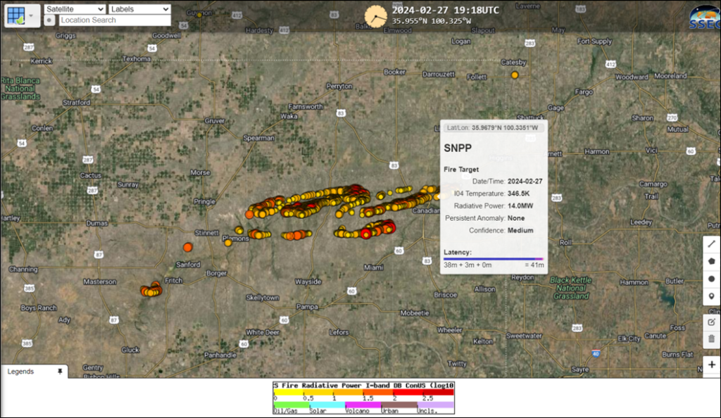
A quantitative VIIRS Active Fires product (accessed online via RealEarth) observed the fire intensities, expressed in MegaWatts (MW). The fire pixels are color coded from yellow to orange to red to dark red colors, where red and dark red colors indicate the most intense fires. Refer to the SNPP VIIRS product image below that shows the fire intensities at ~1918Z, 27 February 2024.

Nighttime visible imagery from the VIIRS NCC product also captured the emitted lights from the fires on 28 February at 0740Z and 0830Z. The emitted lights from the fires are seen within the white ellipse in the Texas Panhandle.

Users can differentiate between the emitted lights from the fires and the emitted lights from the cities / towns by comparing the VIIRS 3.74 um with the nighttime visible imagery. See the animation below. Within the white ellipse, users can identify the warm brightness temperatures in the VIIRS 3.74 um that align with the emitted lights in the VIIRS NCC product. Note, emitted lights that do not have a corresponding thermal signature in the VIIRS 3.74 um, are identified as city or town lights (e.g., Amarillo, TX).

Posted in: Fire Weather, GOES, POES, VIIRS, | Comments closed